User Guide
What is pyvale?
Pyvale is a virtual engineering laboratory that allows you to analyse sensor deployments, optimise experimental design and calibrate/validate simulations. The motivation behind pyvale is to provide engineers with a software tool that they can import a physics simulation and design a simulation validation experiment without needing to go to the laboratory.
Pyvale will never completely replace the need to obtain real experimental data to validate engineering physics simulations. What it can do is reduce the time and cost of experiments by allowing you to perform smarter and more resilient experiments - while providing you the tools to analyse your experimental data to calibrate your simulation or calculate validation metrics.
Another key motivation for pyvale was to provide open-source tools for simulating imaging sensors (e.g. digital image correlation and infra-red thermography) that could be used for large parallel sweeps on computing clusters without licensing restrictions or the need to build from source. With pyvale we aim to make it easy for experimentalists and simulation engineers to simulate their imaging experiments with a simple python interface and underlying performant code.
At the moment we are developing the sensor simulation toolbox for pyvale with a focus on developing our imaging sensor simulation capability (particularly for digital image correlation). In the future we will be adding modules focused on: 1) sensor placement optimisation and experimental design; and 2) simulation calibration and calculating validation metrics.
How does pyvale work?
From a user perspective?
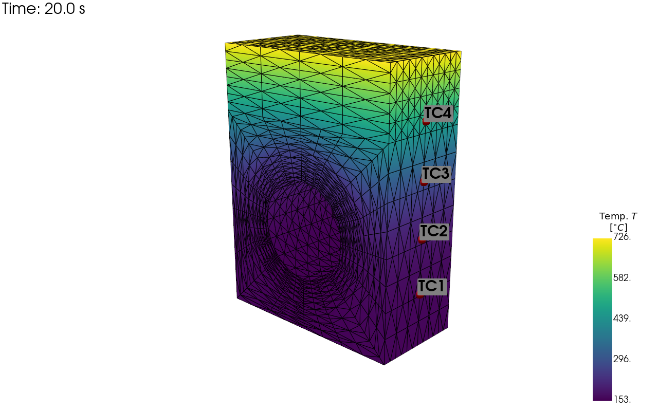
The user workflow for pyvale consists of four main steps: 1) load multi-physics simulation data; 2) build virtual sensor arrays; 3) run simulated experiments; and 4) visualise and analyse the results. We walk through a simple example below for each of these steps. Note that this is a simplified version of the last example in the basics examples.
1. Load multi-physics simulation data.
import numpy as np
import matplotlib.pyplot as plt
import pyvale.mooseherder as mh
import pyvale as pyv

sim_path = pyv.DataSet.thermomechanical_3d_path()
sim_data = mh.ExodusReader(sim_path).read_all_sim_data()
sim_data = pyv.scale_length_units(scale=1000.0,
                                  sim_data=sim_data)
2. Build virtual sensor arrays:
Create sensor positions and sampling times.
x_lims = (12.5,12.5)
y_lims = (0.0,33.0)
z_lims = (0.0,12.0)
n_sens = (1,4,1)
tc_sens_pos = pyv.create_sensor_pos_array(n_sens,x_lims,y_lims,z_lims)

sample_times = np.linspace(0.0,np.max(sim_data.time),50)

tc_sens_data = pyv.SensorData(positions=tc_sens_pos,
                              sample_times=sample_times)
Create the sensor array:
tc_array = pyv.SensorArrayFactory \
 .thermocouples_no_errs(sim_data,
                        tc_sens_data,
                        elem_dims=3,
                        field_name="temperature")
Add some sensor errors to simulate:
tc_err_chain = []
tc_err_chain.append(pyv.ErrSysUnifPercent(low_percent=1.0,high_percent=1.0))
tc_err_chain.append(pyv.ErrRandNormPercent(std=1.0))
tc_error_int = pyv.ErrIntegrator(tc_err_chain,
                                tc_sens_data,
                                tc_array.get_measurement_shape())
tc_array.set_error_integrator(tc_error_int)
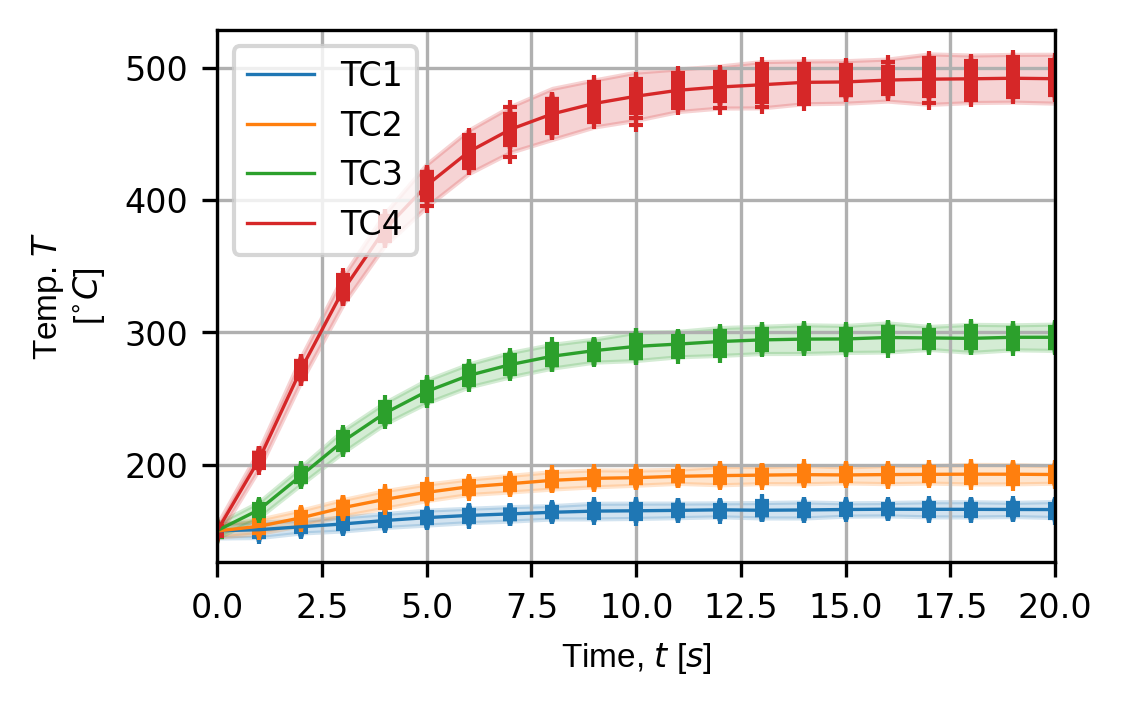
3. Run simulated experiments.
exp_sim = pyv.ExperimentSimulator([sim_data,],
                                  [tc_array,],
                                  num_exp_per_sim=100)

exp_data = exp_sim.run_experiments()
exp_stats = exp_sim.calc_stats()
4. Visualise and analyse results.
pv_plot = pyv.plot_point_sensors_on_sim(tc_array,"temperature")
pv_plot.show()

(fig,ax) = pyv.plot_exp_traces(exp_sim,
                               component="temperature",
                               sens_array_num=0,
                               sim_num=0)
plt.show()
What goes on under the hood?
The core sensor simulation engine in pyvale leverages a suite of scientific computing packages in python including: numpy, scipy, matplotlib and pyvista. All computations that are performed by pyvale in python are implemented as vectorised operations on numpy arrays to improve performance. The results from pyvale sensor simulations are returned as numpy arrays allowing for interoperability with tools like matplotlib for visualisation and scipy for statistical analysis.
For the computationally expensive modules in pyvale such as the simulation of imaging sensors and processing of imaging data (e.g. digital image correlation) we use compiled code that only has minimal interaction with the python interpreter. Note that our imaging simulation and digital image correlation algorithms are still under developement. This means that the user can setup and run a ray-tracing simulation for digital image correlation and then perform digital image correlation on the generated images with only a few lines of python code while maintaining good performance.
How do I get started with pyvale?
You can install pyvale from PyPI using pip install pyvale. We recommend a virtual environment with python 3.11. If you are a new python user and need help setting up the correct python version and your virtual environment then go to our detailed install guide.
Once you have pyvale installed you should get familiar with the core concepts of pyvale starting with the basic examples. These examples come with some pre-packaged simulation data so you will not need to provide your own simulation to get started. With the core functionality of pyvale you will have everything you need to be able to build any custom sensor array that samples scalar (e.g. temperature), vector (e.g. displacement, velocity) or tensor fields (e.g. strain).
After that you might want to look at some of the camera sensor simulation tools in pyvale including our digital image correlation rendering module (based on Blender) and our digital image correlation processing (which are still under developement).
Creating your own sensor models
While we have built and tested pyvale primarily with thermal and solid mechanics problems the interfaces for building sensor simulation models in pyvale are physics agnostic. A sensor is just something that samples a scalar, vector or tensor field at the given locations and given times. This means it is possible to expand on the existing sensor models in pyvale to apply to your own use case such as: velocity or pressure field measurements in fluid mechanics or neutron flux spectrums for neutronics experiments with radiation foils. To help users in setting up their own custom sensor models for their specific physics case we have prepared this guide on custom sensors.
To use pyvale with your own input physics simulation you wil first also need to parse the simulation data into a SimData object. At the moment we support reading the exodus output format (.e) as this is what is generated by the open-source finite element framework we use called MOOSE (Multi-physics Object Oriented Simulation Enviroment). If you need help converting your simulation data please raise an issue on our github page as we are looking to expand the range of common simulation tools we support.
Why is there a rabbit on our logo?
We like rabbits and we like digital image correlation - so a rabbit with a speckle pattern seemed like a good idea. Do we need another reason?
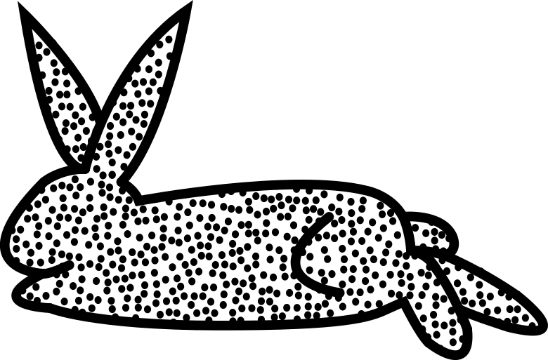
We could have said it was some forced metaphor that rabbits multiply a lot and one of the main applications of pyvale is running large parallel sweeps on computing clusters. But it was actually just a series of jokes from different team members. Someone said “I can’t design the logo because if I do it will have a rabbit on it”, then someone else said that “A rabbits ears look like the ‘V’ in pyvale”. And that was how our logo was born.