2D Plate with a Hole

This example walks through setting up a DIC and strain calculation for the classic “plate with a hole” problem. The images used are synthetically generated, allowing for comparison to analytically known values.

import matplotlib.pyplot as plt
from pathlib import Path

# pyvale modules
import pyvale.dataset as dataset
import pyvale.dic as dic

We’ll start by defining some variables that will be reused throughout the example: the reference image, deformed image(s), and the subset size.

If you’re working with a series of deformed images, it’s a good idea to place them in a separate folder or ensure they follow a consistent naming convention. In such cases, the wildcard operator * can be used to select multiple files.

The images used here are included in the data folder. We’ve provided helper functions to load them regardless of your installation path.

subset_size = 31
ref_img = dataset.dic_plate_with_hole_ref()
def_img = dataset.dic_plate_with_hole_def()

# create a directory for the the different outputs
output_path = Path.cwd() / "pyvale-output"
if not output_path.is_dir():
    output_path.mkdir(parents=True, exist_ok=True)

Next, we’ll select our Region of Interest (ROI) using the interactive tool. Create an instance of the ROI class and pass the reference image as input. This image will be shown as the underlay during any ROI selection or visualization.

roi = dic.RegionOfInterest(ref_img)
roi.interactive_selection(subset_size)

Once you’ve closed the ROI interactive window, a mask and seed location coordinates will be generated. These are needed for the DIC engine.

If you intend to reuse this ROI, it’s a good idea to save it. For large images, setting binary=True is recommended to reduce file size and write time.

roi_file = output_path / "roi.dat"
roi.save_array(filename=roi_file, binary=False)

To load a previously saved ROI for future use, use the read_array method. Make sure the filename and format (binary or human-readable) match what was saved.

roi.read_array(filename=roi_file, binary=False)

Now we can run the 2D DIC engine using pyvale.dic_2d().

This function accepts many optional arguments — consult the documentation for full details. At a minimum, you’ll need to specify:

• Reference image

• Deformed image(s)

• ROI mask

• Seed coordinates (If using a Reliability Guided approach)

• Subset size

By default, the engine uses an affine shape function with the Zero Normalised Sum of Squared Differences (ZNSSD) correlation criterion.

At present, the DIC engine doesn’t return any results to the user, instead the results are saved to disk. You can customize the filename, location, format, and delimiter using the options options output_basepath, output_prefix, output_delimiter, and output_binary. More info on these options can be found in the documentation for dic.two_dimensional(). By default, the results will be saved with the prefix dic_results_ followed by the original filename. The file extension will be replaced will either “.csv” or “dic2d” depending on whether the results are being saved in human-readable or binary format.

dic.two_dimensional(reference=ref_img,
                    deformed=def_img,
                    roi_mask=roi.mask,
                    seed=roi.seed,
                    subset_size=subset_size,
                    subset_step=10,
                    shape_function="AFFINE",
                    max_displacement=10,
                    correlation_criteria="ZNSSD",
                    output_basepath=output_path,
                    output_delimiter=",",
                    output_prefix="dic_results_")

If you saved the results in a human-readable format, you can use any tool (e.g., Excel, Python, MATLAB) for post-processing.

For convenience, we provide a utility function to import results back into Python for analysis and visualization: pyvale.dic_data_import().

The returned object is an instance of pyvale.DICResults. If the results were saved in binary format or with a custom delimiter, be sure to specify those parameters.

dic_files = output_path / "dic_results_*.csv"
dicdata = dic.data_import(data=dic_files, delimiter=",", binary=False)

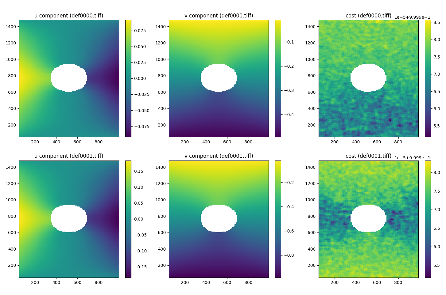
As an example, here’s a simple visualization of the displacement (u, v) and correlation cost for the two deformed images using matplotlib. You’ll need to ensure you have matplotlib.pyplot installed and imported.

fig, axes = plt.subplots(2, 3, figsize=(15, 5))
axes = axes.flatten()

# First deformation image
im1 = axes[0].pcolor(dicdata.ss_x, dicdata.ss_y, dicdata.u[0])
im2 = axes[1].pcolor(dicdata.ss_x, dicdata.ss_y, dicdata.v[0])
im3 = axes[2].pcolor(dicdata.ss_x, dicdata.ss_y, dicdata.cost[0])

# Second deformation image
im4 = axes[3].pcolor(dicdata.ss_x, dicdata.ss_y, dicdata.u[1])
im5 = axes[4].pcolor(dicdata.ss_x, dicdata.ss_y, dicdata.v[1])
im6 = axes[5].pcolor(dicdata.ss_x, dicdata.ss_y, dicdata.cost[1])

# Titles
axes[0].set_title('u component (def0000.tiff)')
axes[1].set_title('v component (def0000.tiff)')
axes[2].set_title('cost (def0000.tiff)')
axes[3].set_title('u component (def0001.tiff)')
axes[4].set_title('v component (def0001.tiff)')
axes[5].set_title('cost (def0001.tiff)')

# Colorbars
fig.colorbar(im1, ax=axes[0])
fig.colorbar(im2, ax=axes[1])
fig.colorbar(im3, ax=axes[2])
fig.colorbar(im4, ax=axes[3])
fig.colorbar(im5, ax=axes[4])
fig.colorbar(im6, ax=axes[5])

plt.tight_layout()
plt.show()