Errors: calibration

In this example we show how pyvale can simulate sensor calibration errors with user defined calibration functions.

from pathlib import Path
import numpy as np
import matplotlib.pyplot as plt

# pyvale imports
import pyvale.mooseherder as mh
import pyvale.sensorsim as sens
import pyvale.dataset as dataset

Calibration Functions

First we need to define some calibration functions. These functions must take a numpy array and return a numpy array of the same shape. We start by defining what we think our calibration is called calib_assumed() and then we also need to define the ground truth calibration calib_truth() so that we can calculate the error between them. The calibration functions shown below are simplified versions of the typical calibration curves for a K-type thermocouple.

def calib_assumed(signal: np.ndarray) -> np.ndarray:
    return 24.3*signal + 0.616


def calib_truth(signal: np.ndarray) -> np.ndarray:
    return -0.01897 + 25.41881*signal - 0.42456*signal**2 + 0.04365*signal**3

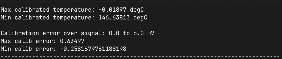
We are first going to do a quick analytical calculation for the minimum and maximum systematic error we expect between our assumed and true calibration. For our true calibration we know this holds between 0 and 6mV so we perform the calculation over this range and print the min/max expected error over this range.

n_cal_divs = 10000
signal_calib_range = np.array((0.0,6.0),dtype=np.float64)
milli_volts = np.linspace(signal_calib_range[0],
                            signal_calib_range[1],
                            n_cal_divs)
temp_truth = calib_truth(milli_volts)
temp_assumed = calib_assumed(milli_volts)
calib_error = temp_assumed - temp_truth

print()
print(80*"-")
print(f"Max calibrated temperature: {np.min(temp_truth)} degC")
print(f"Min calibrated temperature: {np.max(temp_truth)} degC")
print()
print(f"Calibration error over signal:"
        + f" {signal_calib_range[0]} to {signal_calib_range[1]} mV")
print(f"Max calib error: {np.max(calib_error)}")
print(f"Min calib error: {np.min(calib_error)}")
print(80*"-")
print()

1. Load physics simulation data

data_path: Path = dataset.thermal_2d_path()
sim_data: mh.SimData = mh.ExodusLoader(data_path).load_all_sim_data()
sim_data: mh.SimData = sens.scale_length_units(scale=1000.0,
                                               sim_data=sim_data,
                                               disp_keys=None)

2. Build virtual sensor array

sim_dims: dict[str,tuple[float,float]] = sens.simtools.get_sim_dims(sim_data)
sens_pos: np.ndarray = sens.gen_pos_grid_inside(num_sensors=(3,2,1),
                                                x_lims=sim_dims["x"],
                                                y_lims=sim_dims["y"],
                                                z_lims=(0.0,0.0))

sample_times: np.ndarray = np.linspace(0.0,np.max(sim_data.time),50)

sens_data = sens.SensorData(positions=sens_pos,
                            sample_times=sample_times)

sens_array: sens.SensorsPoint = sens.SensorFactory.scalar_point(
    sim_data,
    sens_data,
    comp_key="temperature",
    spatial_dims=sens.EDim.TWOD,
    descriptor=sens.DescriptorFactory.temperature(),
)

2.1. Add simulated measurement errors

With our assumed and true calibration functions we can build our calibration error object and add it to our error chain as normal. Note that the truth calibration function must be inverted numerically so to increase accuracy the number of divisions can be increased. However, 1e4 divisions should be suitable for most applications.

cal_err = sens.ErrSysCalibration(calib_assumed,
                                 calib_truth,
                                 signal_calib_range,
                                 n_cal_divs=10000)
sens_array.set_error_chain([cal_err,])

3. Run a simulated experiment

measurements = sens_array.sim_measurements()

print(80*"-")

sens_print = 0
comp_print = 0
time_last = 5
time_print = slice(measurements.shape[2]-time_last,measurements.shape[2])

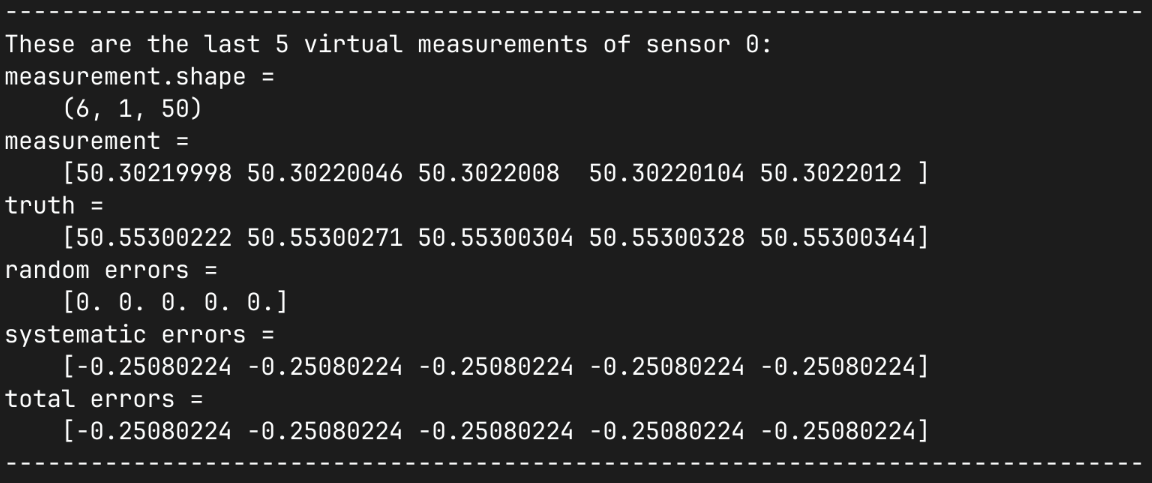
print(f"These are the last {time_last} virtual measurements of sensor "
        + f"{sens_print}:")

sens.print_measurements(sens_array,sens_print,comp_print,time_print)

print(80*"-")

4. Visualise the results

output_path = Path.cwd() / "pyvale-output"
if not output_path.is_dir():
    output_path.mkdir(parents=True, exist_ok=True)

(fig,ax) = sens.plot_time_traces(sens_array,comp_key="temperature")
save_traces = output_path/"ext_ex4f_traces.png"
fig.savefig(save_traces, dpi=300, bbox_inches="tight")

# Uncomment this to display the sensor trace plot
# plt.show()