Multi-physics experiment simulation

In this example we apply multiple sensor arrays across a number of different physics simulations with different inputs allowing us to run a series of virtual experiments and analyse the results.

from pathlib import Path
import numpy as np
import matplotlib.pyplot as plt

# pyvale imports
import pyvale.mooseherder as mh
import pyvale.sensorsim as sens
import pyvale.dataset as dataset

1. Load physics simulation data

First we load a set of simulations all of the same thermo-mechanical test case where one simulation uses the reference thermal conductivity and expansion coefficient and the remaining simulation represents a -10% perturbation to these simulation inputs.

sim_paths: list[Path] = dataset.thermomechanical_3d_experiment_paths()
sim_keys: set[str] = {"sim_nominal","sim_perturbed"}

disp_keys = ("disp_x","disp_y","disp_z")

sim_data_dict: dict[str,mh.SimData] = {}
for ss,kk in zip(sim_paths,sim_keys):
    sim_data: mh.SimData = mh.ExodusLoader(ss).load_all_sim_data()

    sim_data: mh.SimData = sens.scale_length_units(scale=1000.0,
                                                   sim_data=sim_data,
                                                   disp_keys=disp_keys)
    sim_data_dict[kk] = sim_data

2. Build virtual sensor arrays

2.1 Build scalar field sensor array

Here we build a scalar field sensor array to simulate thermocouples applied to our simulation in a similar way to what we have seen in previous examples.

sample_times = np.linspace(0.0,np.max(sim_data.time),50)

temp_sens_pos: np.ndarray = sens.gen_pos_grid_inside(num_sensors=(1,4,1),
                                                     x_lims=(12.5,12.5),
                                                     y_lims=(0.0,33.0),
                                                     z_lims=(0.0,12.0))

temp_sens_data = sens.SensorData(positions=temp_sens_pos,
                                 sample_times=sample_times)

temp_sens: sens.SensorsPoint = sens.SensorFactory.scalar_point(
    sim_data,
    temp_sens_data,
    comp_key="temperature",
    spatial_dims=sens.EDim.THREED,
    descriptor=sens.DescriptorFactory.temperature(),
)

2.2 Add errors to the scalar field sensors

Now we add some errors to our thermocouple sensor array starting with a random noise with a standard deviation of 2 degrees. We then build a field error that includes sensor position uncertainty. Here we generate position uncertainty in all dimensions but then we use the pos_lock_xyz numpy array in our ErrFieldData object to constrain all sensors to not move off the surface they are on. This feature is particularly useful when we have sensors on different faces of a 3D simulation and we want to constrain the sensors in particular axes for particular sensors. However, here we could have just omitted the position random generator in the X direction and replace it with None.

temp_pos_uncert = 0.5 # units = mm
temp_pos_rand = (sens.GenNormal(std=temp_pos_uncert),
                 sens.GenNormal(std=temp_pos_uncert),
                 sens.GenNormal(std=temp_pos_uncert))

temp_pos_lock = np.full(temp_sens_pos.shape,False,dtype=bool)
temp_pos_lock[:,0] = True

temp_field_err_data = sens.ErrFieldData(pos_rand_xyz=temp_pos_rand,
                                        pos_lock_xyz=temp_pos_lock)

temp_err_chain: list[sens.IErrSimulator] = [
    sens.ErrRandGen(sens.GenNormal(std=2.0)), # units = degrees
    sens.ErrSysField(temp_sens.get_field(),temp_field_err_data),
]

temp_sens.set_error_chain(temp_err_chain)

2.3 Build tensor field sensor array

Here we build a tensor field sensor array to simulate strain gauges applied to our simulation in a similar way to what we have seen in previous examples.

strain_sens_pos: np.ndarray = sens.gen_pos_grid_inside(num_sensors=(1,4,1),
                                                       x_lims=(9.4,9.4),
                                                       y_lims=(0.0,33.0),
                                                       z_lims=(12.0,12.0))

strain_sens_data = sens.SensorData(positions=strain_sens_pos,
                                   sample_times=sample_times)

strain_sens: sens.SensorsPoint = sens.SensorFactory.tensor_point(
    sim_data,
    strain_sens_data,
    norm_comp_keys=("strain_xx","strain_yy","strain_zz"),
    dev_comp_keys=("strain_xy","strain_yz","strain_xz"),
    spatial_dims=sens.EDim.THREED,
    descriptor=sens.DescriptorFactory.strain(sens.EDim.THREED),
)

2.4 Add errors to the tensor field sensors

Now we add some errors to our strain gauge array starting with random noise with a standard deviation of 2% of the ground truth. We then build a field error to simulate orientation uncertainty and demonstrate the same ‘lock’ functionality that allows us to constrain the sensors to only rotate on the surface they are on.

angle_uncert: float = 2.0 # units = degrees
angle_rand_zyx = (sens.GenUniform(low=-angle_uncert,high=angle_uncert),
                  sens.GenUniform(low=-angle_uncert,high=angle_uncert),
                  sens.GenUniform(low=-angle_uncert,high=angle_uncert))

angle_lock = np.full(strain_sens_pos.shape,True,dtype=bool)
angle_lock[:,0] = False   # Allow rotation about z

strain_field_err_data = sens.ErrFieldData(ang_rand_zyx=angle_rand_zyx,
                                          ang_lock_zyx=angle_lock)

strain_err_chain: list[sens.IErrSimulator] = [
    sens.ErrRandGenPercent(sens.GenNormal(std=2.0)),
    sens.ErrSysField(strain_sens.get_field(),strain_field_err_data),
]

strain_sens.set_error_chain(strain_err_chain)

3. Create & run simulated experiments

We can now run our experiments over all simulations for all our virtual sensor arrays. We can run our simulations sequentially or in parallel by controlling the number of workers and parallelisation enumeration in the ExpSimOpts dataclass. Note that the default is to run the simulations in a single process sequentially (called the ALL option). The parallelisation enumeration has two options ‘ALL’ which means we run all of our N experiments on per worker and ‘SPLIT’ which splits our N experiments across the workers running a single simulation per worker. For our case here ‘ALL’ will be fastest and as we have 4 unique combinations of our simulation data and sensors arrays 4 workers will be most efficient. The ‘SPLIT’ option is most effective for computationally heavy simulated experiments that involve imaging simulations.

We can also control what data is saved from our experiment simulation using ExpSimSaveKeys dataclass. Here you can assign custom keys to the different data arrays (measurement, systematic error and random error arrays etc.) or setting any of the member variables of the save keys to None will stop that variable being save. This is useful if you only have systematic errors and no random errors so don’t need to save them (set .rand=None). If you have no field errors perturbing the sensor positon or time you will also want to stop these arrays being saves (.pert_sens_times=None, .pert_sens_pos=None) .

sensor_array_dict: dict[str,sens.ISensorArray] = {
    "temp": temp_sens,
    "strain": strain_sens,
}

exp_sim_opts = sens.ExpSimOpts(workers=4,para=sens.EExpSimPara.ALL)
exp_save_keys = sens.ExpSimSaveKeys(pert_sens_times=None)

exp_sim = sens.ExperimentSimulator(sim_data_dict,
                                   sensor_array_dict,
                                   exp_sim_opts,
                                   exp_save_keys)

The results of our simulated experiment are returned as a dictionary of numpy arrays where the key is a tuple of strings. The tuple key takes the form: (sim_key,sens_key,data_key) where data_key can be: “meas” for the simulated measurements; “sys_errs” for the systematic errors; “rand_errs” for the random errors; and “samp_times” for the sample time vector. The numpy array for “meas”, “sys_errs” and “rand_errs” has the following shape (num_exps,num_sensors,num_field_comps,num_time_steps). The numpy array for the sample times has a shape (num_time_steps,). This will also contain the perturbed sensor positions with data key “pert_sens_pos”. In our case we are not perturbing the sensor times and we have set the save key to None so this will not appear in our data dictionary.

We can also calculate summary statistics which is returned as a dictionary keyed with the same tuple as the experimental data dictionary. The value of dictionary is an experiment stats object that contains numpy arrays for each statistic that is collapsed over the number of simulated experiments. The statistics we can access include: mean, standard deviation minimum, maximum, median, median absolute deviation and the 25% and 75% quartiles. See the ExpSimStats data class for details.

exp_data: dict[tuple[str,...],np.ndarray] = (
    exp_sim.run_experiments(num_exp_per_sim=100)
)
exp_stats: dict[tuple[str,...],sens.ExpSimStats] = (
    sens.calc_exp_sim_stats(exp_data)
)

4. Analyse & visualise the results

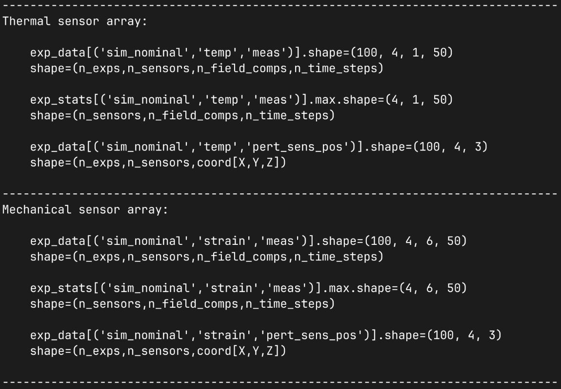
Here we inspect our experiment simulation data dictionary to demonstrate the the data structures it contains so you can perform any follow up analysis on the data you want. We first print the tuple keys in our dictionary so we can see what data is available.

print(80*"-")
print("Keys in the simulated experimental data dictionary:")
for kk in exp_data:
    print(kk)
print(80*"-")
print()

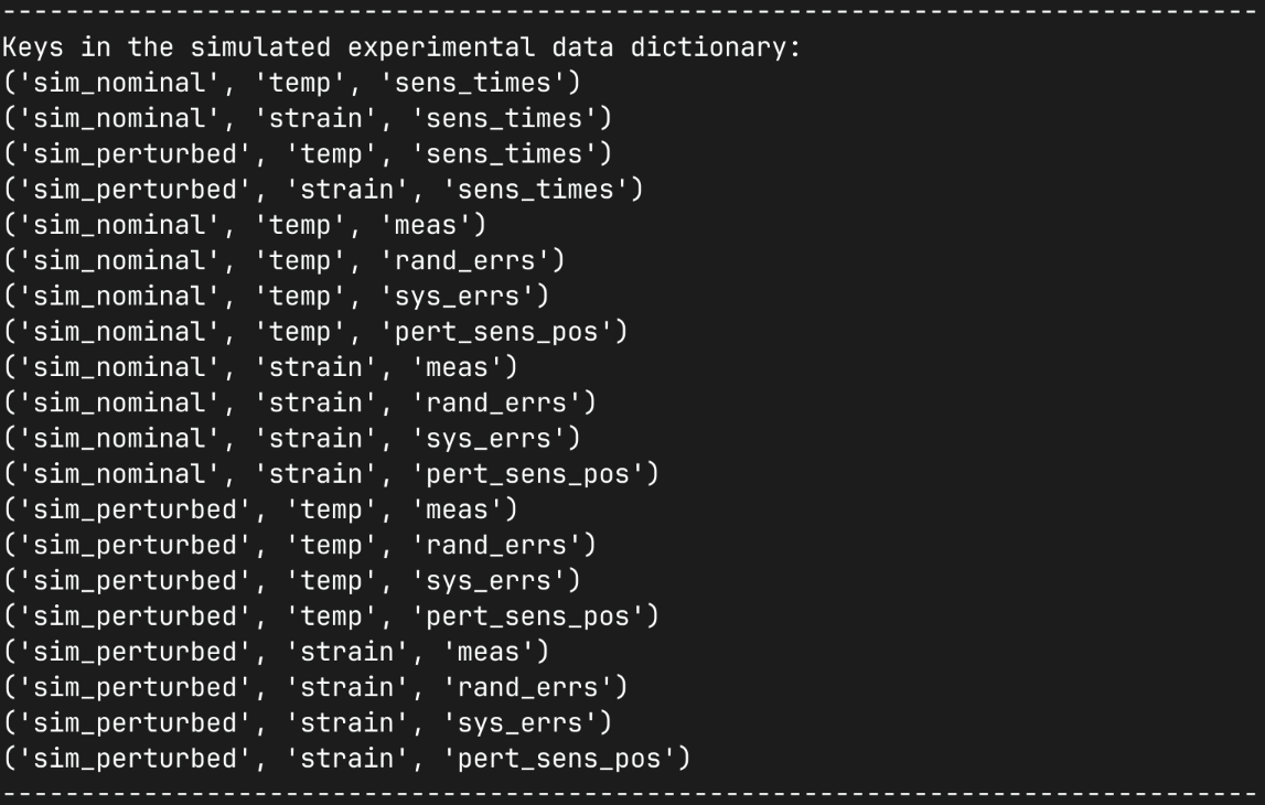
We then inspect the simulated data output for few combinations of simulations and sensor arrays showing the shapes of the raw data arrays and the calculated statistics. Noting that our scalar field sensor has a differen number of component dimensions to our mechanical field sensor.

print(80*"-")
print("Thermal sensor array:")
print()
print(f"    {exp_data[('sim_nominal','temp','meas')].shape=}")
print("    shape=(n_exps,n_sensors,n_field_comps,n_time_steps)")
print()
print(f"    {exp_stats[('sim_nominal','temp','meas')].max.shape=}")
print("    shape=(n_sensors,n_field_comps,n_time_steps)")
print()
print(f"    {exp_data[('sim_nominal','temp','pert_sens_pos')].shape=}")
print("    shape=(n_exps,n_sensors,coord[X,Y,Z])")
print()
print(80*"-")
print("Mechanical sensor array:")
print()
print(f"    {exp_data[('sim_nominal','strain','meas')].shape=}")
print("    shape=(n_exps,n_sensors,n_field_comps,n_time_steps)")
print()
print(f"    {exp_stats[('sim_nominal','strain','meas')].max.shape=}")
print("    shape=(n_sensors,n_field_comps,n_time_steps)")
print()
print(f"    {exp_data[('sim_nominal','strain','pert_sens_pos')].shape=}")
print("    shape=(n_exps,n_sensors,coord[X,Y,Z])")
print()
print(80*"-")

We can save the output experiment simulation data dicitionary to disk and load it using the save_exp_sim_data and load_exp_sim_data functions. First, we create the standard pyvale output directory in your current working directory so we can save our data there.

output_path: Path = Path.cwd() / "pyvale-output"
if not output_path.is_dir():
    output_path.mkdir(parents=True, exist_ok=True)

sens.save_exp_sim_data(output_path/"ex3_exp_sim_data.npz",exp_data)

exp_data: dict[tuple[str,...],np.ndarray] = sens.load_exp_sim_data(
    output_path/"ex3_exp_sim_data.npz"
)

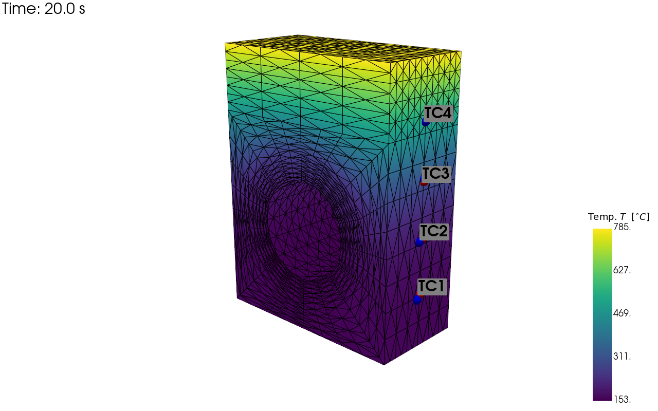
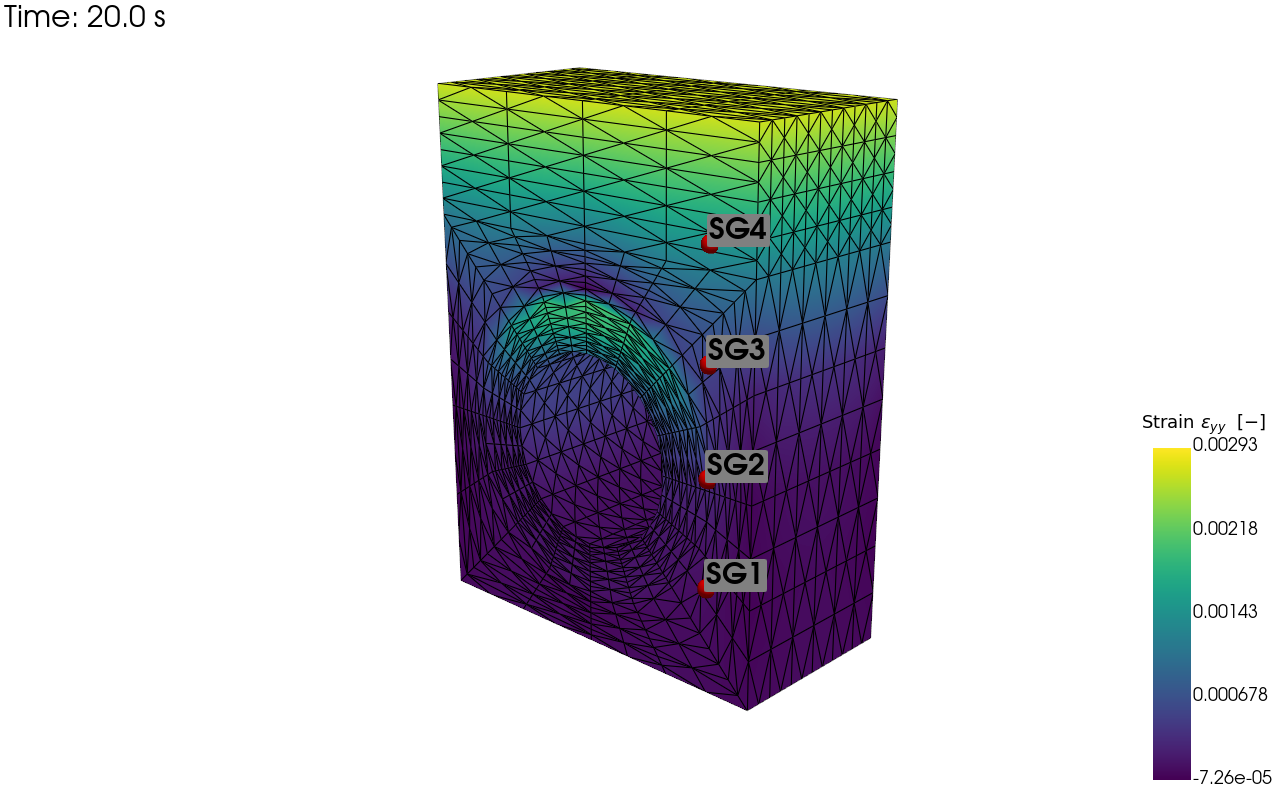
Now we are going to save visualisations of our temperature and strain sensor locations on the simulation mesh so we can verify we have setup their locations as we expected.

cam_pos = np.array([(59.354, 43.428, 69.946),
                    (-2.858, 13.189, 4.523),
                    (-0.215, 0.948, -0.233)])

pv_plot = sens.plot_point_sensors_on_sim(temp_sens,"temperature")
pv_plot.camera_position = cam_pos

# Set to False to show an interactive plot instead of saving the figure
pv_plot.off_screen = True
if pv_plot.off_screen:
    pv_plot.screenshot(output_path/"basics_ex3_temp_locs.png")
else:
    pv_plot.show()

Visualisation of the virtual temperature sensor locations:

pv_plot = sens.plot_point_sensors_on_sim(strain_sens,"strain_yy")
pv_plot.camera_position = cam_pos

# Set to False to show an interactive plot instead of saving the figure
pv_plot.off_screen = True
if pv_plot.off_screen:
    pv_plot.screenshot(output_path/"basics_ex3_strain_locs.png")
else:
    pv_plot.show()

Visualisation of the virtual strain sensor locations:

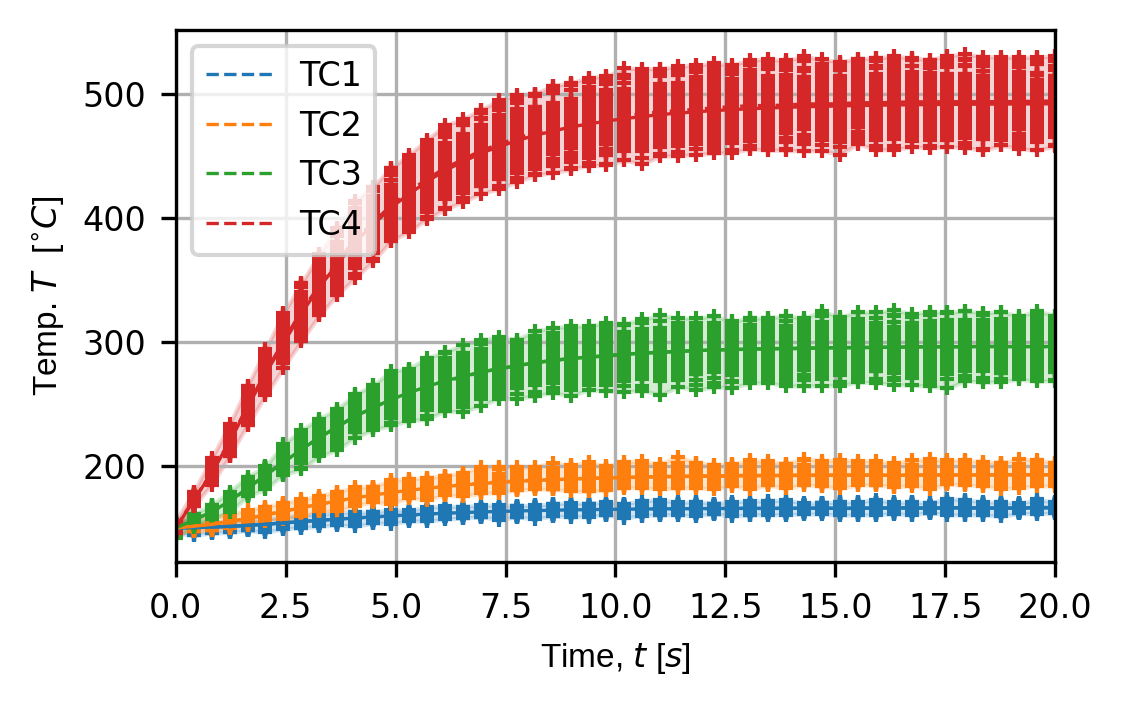
Finally, we plot the traces for all simulated experiments for our virtual temperature and strain sensors.

trace_opts = sens.TraceOptsExperiment(plot_all_exp_points=True)

(fig,ax) = sens.plot_exp_traces(
    exp_data,
    comp_ind=0,
    sens_key="temp",
    sim_key="sim_nominal",
    trace_opts=trace_opts,
    descriptor=sens.DescriptorFactory.temperature(),
)

save_fig: Path = output_path/"basics_ex3_traces_temp.png"
fig.savefig(save_fig,dpi=300,bbox_inches="tight")

Virtual temperature sensor traces over all simulated experiments for the nominal input simulation:

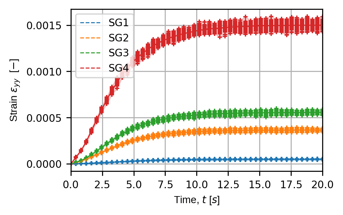
strain_plot_keys = ("strain_xx","strain_yy","strain_xy")
for ii,kk in enumerate(strain_plot_keys):
    (fig,ax) = sens.plot_exp_traces(
        exp_data,
        comp_ind=ii,
        sens_key="strain",
        sim_key="sim_nominal",
        trace_opts=trace_opts,
        descriptor=sens.DescriptorFactory.strain(sens.EDim.THREED),
    )

    save_fig: Path = output_path/f"basics_ex3_traces_{kk}.png"
    fig.savefig(save_fig,dpi=300,bbox_inches="tight")

Virtual strain sensor traces over all simulated experiments for the perturbed input simulation:

# Uncomment this to display the sensor trace plots
# plt.show()