Errors: spatial averaging

In this example we show how pyvale can simulate sensor spatial averaging for ground truth calculations as well as for calculating systematic errors.

from pathlib import Path
import numpy as np
import matplotlib.pyplot as plt

# pyvale imports
import pyvale.mooseherder as mh
import pyvale.sensorsim as sens
import pyvale.dataset as dataset

1. Load physics simulation data

data_path: Path = dataset.thermal_2d_path()
sim_data: mh.SimData = mh.ExodusLoader(data_path).load_all_sim_data()
sim_data: mh.SimData = sens.scale_length_units(scale=1000.0,
                                               sim_data=sim_data,
                                               disp_keys=None)

2. Build virtual sensor arrays

Now we are going to build a scalar field sensor array so we can control how the ground truth is extracted for a sensor using area averaging. Note that the default is an ideal point sensor with no spatial averaging. Later we will add area averaging as a systematic error. Note that it is possible to have an ideal point sensor with no area averaging for the truth and then add an area averaging error. It is also possible to have a truth that is area averaged without and area averaging error. Finally, you can specify different averaging areas for the truth and systematic errors.

sim_dims: dict[str,tuple[float,float]] = sens.simtools.get_sim_dims(sim_data)
sens_pos: np.ndarray = sens.gen_pos_grid_inside(num_sensors=(3,2,1),
                                                x_lims=sim_dims["x"],
                                                y_lims=sim_dims["y"],
                                                z_lims=(0.0,0.0))

sample_times: np.ndarray = np.linspace(0.0,np.max(sim_data.time),50)

This is where we control the setup of the area averaging. We need to specify the sensor dimensions and the type of numerical spatial integration to use. Here we specify a square sensor in x and y with 4 point Gaussian quadrature integration. It is worth noting that increasing the number of integration points will increase computational cost as each additional integration point requires an additional interpolation of the physical field.

sensor_dims = np.array([5.0,5.0,0]) # units = mm

sens_data = sens.SensorData(positions=sens_pos,
                            sample_times=sample_times,
                            spatial_averager=sens.EIntSpatialType.QUAD4PT,
                            spatial_dims=sensor_dims)

We have added spatial averaging to our sensor data so we can now create our sensor array as we have done in previous examples.

sens_array: sens.SensorsPoint = sens.SensorFactory.scalar_point(
    sim_data,
    sens_data,
    comp_key="temperature",
    spatial_dims=sens.EDim.TWOD,
    descriptor=sens.DescriptorFactory.temperature(),
)

2.1. Add simulated measurement errors

We are going to create a field error that includes area averaging as an error. We do this by adding the option to our field error data class specifying rectangular integration with 1 point.

area_avg_err_data = sens.ErrFieldData(
    spatial_averager=sens.EIntSpatialType.RECT1PT,
    spatial_dims=np.array((20.0,20.0)),
)

We add the field error to our error chain as normal. We could combine it with any of our other error models but we will isolate it for now so we can see what it does.

err_chain: list[sens.IErrSimulator] = [
    sens.ErrSysField(sens_array.get_field(),area_avg_err_data),
]

sens_array.set_error_chain(err_chain)

3. Run a simulated experiment

Now we run our sensor simulation to see how spatial averaging changes our simulated measurement results.

measurements = sens_array.sim_measurements()

print(80*"-")
sens_print = 0
comp_print = 0
time_last = 5
time_print = slice(measurements.shape[2]-time_last,measurements.shape[2])

print(f"These are the last {time_last} virtual measurements of sensor "
        + f"{sens_print}:")

sens.print_measurements(sens_array,sens_print,comp_print,time_print)
print(80*"-")

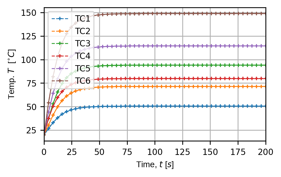
4. Visualise the results

output_path = Path.cwd() / "pyvale-output"
if not output_path.is_dir():
    output_path.mkdir(parents=True, exist_ok=True)

(fig,ax) = sens.plot_time_traces(sens_array,comp_key="temperature")
save_traces = output_path/"ext_ex4g_traces.png"
fig.savefig(save_traces, dpi=300, bbox_inches="tight")

# Uncomment this to display the sensor trace plot
# plt.show()