Tensor field sensors in 2D

This example demonstrates the application of the pyvale sensor simulation module to tensor fields in 2 spatial dimensions. An example of a vector field sensor would be a displacement transducer, point tracking or velocity sensor.

Note that this example has minimal explanation and assumes you have reviewed the basic sensor simulation examples to understand how the underlying engine works as well as the sensor simulation workflow.

from pathlib import Path
import numpy as np
import matplotlib.pyplot as plt
from scipy.spatial.transform import Rotation

# pyvale imports
import pyvale.mooseherder as mh
import pyvale.sensorsim as sens
import pyvale.dataset as dataset

1. Load physics simulation data

data_path: Path = dataset.mechanical_2d_path()
sim_data: mh.SimData = mh.ExodusLoader(data_path).load_all_sim_data()

disp_keys = ("disp_x","disp_y")
norm_comp_keys = ("strain_xx","strain_yy")
dev_comp_keys = ("strain_xy",)

sim_data: mh.SimData = sens.scale_length_units(scale=1000.0,
                                               sim_data=sim_data,
                                               disp_keys=("disp_x","disp_y"))

2. Build virtual sensor arrays

sim_dims: dict[str,tuple[float,float]] = sens.simtools.get_sim_dims(sim_data)
sens_pos: np.ndarray = sens.gen_pos_grid_inside(num_sensors=(2,2,1),
                                                x_lims=sim_dims["x"],
                                                y_lims=sim_dims["y"],
                                                z_lims=(0.0,0.0))

sample_times: np.ndarray = np.linspace(0.0,np.max(sim_data.time),50)

sens_angles: tuple[Rotation] = (
    Rotation.from_euler("zyx",[0,0,0], degrees=True),
)

sens_data = sens.SensorData(positions=sens_pos,
                            sample_times=sample_times,
                            angles=sens_angles)

descriptor = sens.SensorDescriptor(name="Strain",
                                   symbol=r"\varepsilon",
                                   units=r"-",
                                   tag="SG",
                                   components=("xx","yy","xy"))

sens_array: sens.SensorsPoint = sens.SensorFactory.tensor_point(
    sim_data,
    sens_data,
    norm_comp_keys=norm_comp_keys,
    dev_comp_keys=dev_comp_keys,
    spatial_dims=sens.EDim.TWOD,
    descriptor=descriptor,
)

2.1. Add simulated measurement errors

pos_rand = sens.GenUniform(low=-1.0,high=1.0)   # units = mm
angle_rand = sens.GenUniform(low=-2.0,high=2.0) # units = degrees

field_err_data = sens.ErrFieldData(pos_rand_xyz=(pos_rand,pos_rand,None),
                                   ang_rand_zyx=(angle_rand,None,None))

error_chain: list[sens.IErrSimulator] = [
    sens.ErrSysGenPercent(sens.GenUniform(low=-1.0,high=1.0)),
    sens.ErrRandGenPercent(sens.GenNormal(std=1.0)),
    sens.ErrSysField(sens_array.get_field(),field_err_data),
]

sens_array.set_error_chain(error_chain)

3. Create & run simulated experiment

measurements: np.ndarray = sens_array.sim_measurements()

truth: np.ndarray = sens_array.get_truth()
sys_errs: np.ndarray = sens_array.get_errors_systematic()
rand_errs: np.ndarray = sens_array.get_errors_random()

print(80*"-")
print("measurement = truth + sysematic error + random error")

print(f"measurements.shape = {measurements.shape} = "
        + "(n_sensors,n_field_components,n_timesteps)")
print(f"truth.shape     = {truth.shape}")
print(f"sys_errs.shape  = {sys_errs.shape}")
print(f"rand_errs.shape = {rand_errs.shape}")

sens_print: int = 0
comp_print: int = 1
time_last: int = 5
time_print = slice(measurements.shape[2]-time_last,measurements.shape[2])

print(f"\nThese are the last {time_last} virtual measurements of sensor "
        + f"{sens_print}:\n")

sens.print_measurements(sens_array,sens_print,comp_print,time_print)
print("\n"+80*"-")

4. Analyse & visualise the results

output_path = Path.cwd() / "pyvale-output"
if not output_path.is_dir():
    output_path.mkdir(parents=True, exist_ok=True)

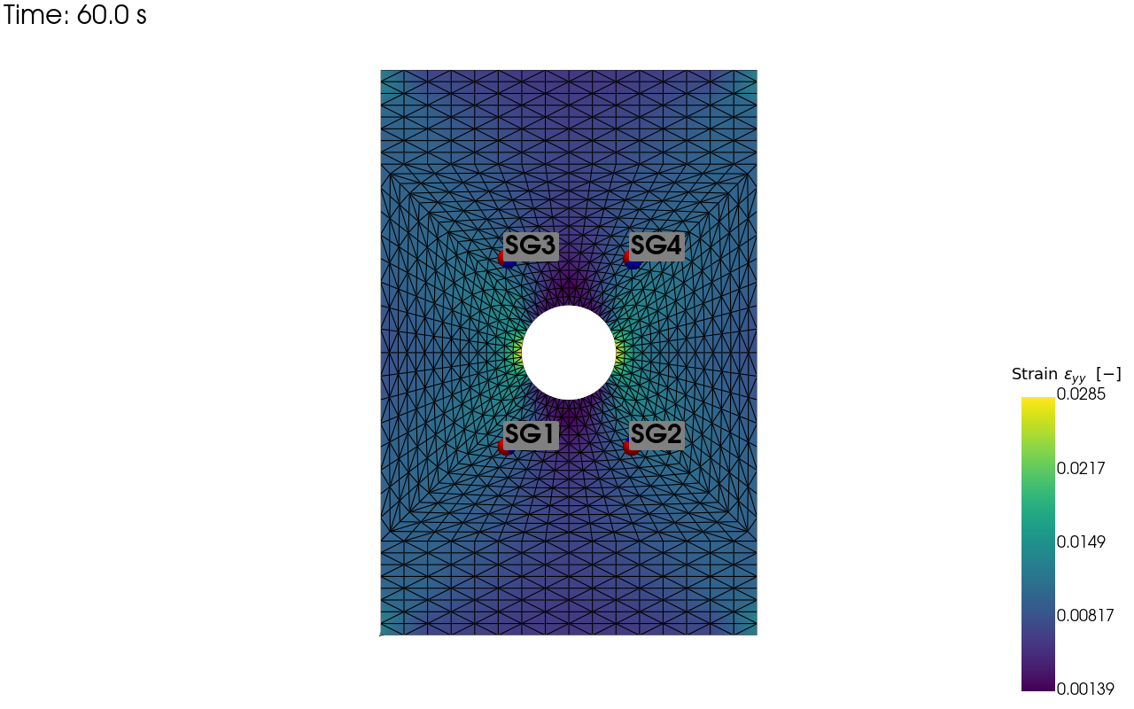
for kk in (norm_comp_keys+dev_comp_keys):
    pv_plot = sens.plot_point_sensors_on_sim(sens_array,kk)
    pv_plot.camera_position = "xy"

    # Set to False to show an interactive plot instead of saving the figure
    pv_plot.off_screen = True
    if pv_plot.off_screen:
        pv_plot.screenshot(output_path/f"ext_ex3e_locs_{kk}.png")
    else:
        pv_plot.show()

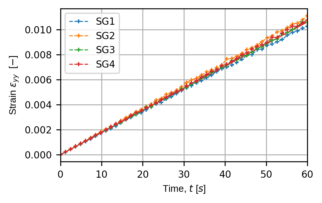
for kk in (norm_comp_keys+dev_comp_keys):
    (fig,ax) = sens.plot_time_traces(sens_array,comp_key=kk)
    fig.savefig(output_path/f"ext_ex3e_traces_{kk}.png",
                dpi=300,
                bbox_inches="tight")

# Uncomment this to display the sensor trace plot
# plt.show()