Strain and Deformation Gradient Calculations

This example follows on from the previous one. It assumes that the DIC results have already been generated in the current working directory and are ready to be used for strain calculations.

import matplotlib.pyplot as plt
from pathlib import Path

# pyvale modules
import pyvale.dic as dic

We’ll start by importing the DIC data from the previous example.

# create a directory for the the different outputs
output_path = Path.cwd() / "pyvale-output"
if not output_path.is_dir():
    output_path.mkdir(parents=True, exist_ok=True)

# specify where our input data is
input_data = output_path / "dic_results_*.csv"

You can calculate strain directly from the DIC results. It’s not necessary to load the data beforehand — you can simply pass the filename (or pattern) to the data argument. If you used a custom delimiter or saved in binary format, make sure to specify those as well.

At a minimum, you need to specify the strain window size and the element type used within the window. The valid options for window_element are:

• 4 for bilinear

• 9 for biquadratic

The output will always include the window coordinates and the full deformation gradient tensor. If you also specify a strain_formulation, the corresponding 2D strain tensor will be included in the output.

dic.strain_two_dimensional(data=input_data, window_size=5, window_element=4,
                           output_basepath=output_path)

Once the strain calculation is complete, you can import the results using pyvale.strain_data_import().

Be sure to specify the delimiter, format (binary or not), and layout.

strain_output = output_path / "strain_dic_results_*.csv"
straindata = dic.strain_data_import(data=strain_output,
                                    binary=False, delimiter=",",
                                    layout="matrix")

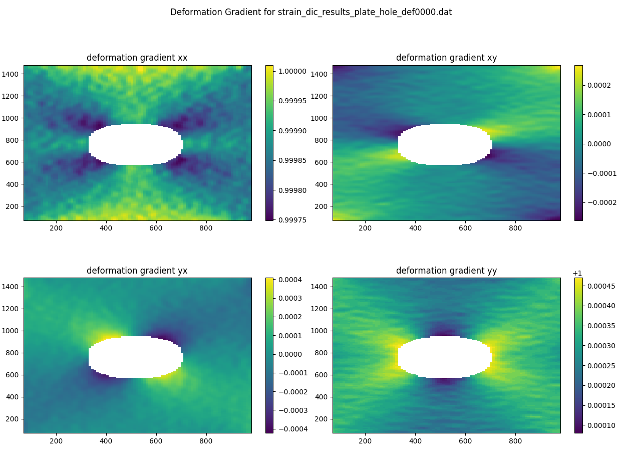
Here’s a simple example of how to visualize the deformation gradient components for the first deformation step using matplotlib.

fig, axes = plt.subplots(2, 2, figsize=(15, 5))
axes = axes.flatten()
fig.suptitle('Deformation Gradient for ' + straindata.filenames[0])

im1 = axes[0].pcolor(straindata.window_x, straindata.window_y, straindata.def_grad[0, :, :, 0, 0])
im2 = axes[1].pcolor(straindata.window_x, straindata.window_y, straindata.def_grad[0, :, :, 0, 1])
im3 = axes[2].pcolor(straindata.window_x, straindata.window_y, straindata.def_grad[0, :, :, 1, 0])
im4 = axes[3].pcolor(straindata.window_x, straindata.window_y, straindata.def_grad[0, :, :, 1, 1])

# titles
axes[0].set_title('deformation gradient xx')
axes[1].set_title('deformation gradient xy')
axes[2].set_title('deformation gradient yx')
axes[3].set_title('deformation gradient yy')

# Colorbars
fig.colorbar(im1, ax=axes[0])
fig.colorbar(im2, ax=axes[1])
fig.colorbar(im3, ax=axes[2])
fig.colorbar(im4, ax=axes[3])

plt.tight_layout()
plt.show()