Errors: field-based

In this example we give an overview of field-based systematic errors. Field errors require additional interpolation of the underlying physical field such as uncertainty in a sensor position or sampling time. For this example we will focus on field error sources that perturb sensor locations and sampling times.

Note that field errors are more computationally intensive than basic errors as they require additional interpolations of the underlying physical field.

from pathlib import Path
import numpy as np
import matplotlib.pyplot as plt

# pyvale imports
import pyvale.mooseherder as mh
import pyvale.sensorsim as sens
import pyvale.dataset as dataset

1. Load physics simulation data

data_path: Path = dataset.thermal_3d_path()
sim_data: mh.SimData = mh.ExodusLoader(data_path).load_all_sim_data()
sim_data: mh.SimData = sens.scale_length_units(scale=1000.0,
                                               sim_data=sim_data,
                                               disp_keys=None)

2. Build virtual sensor array

sim_dims = sens.simtools.get_sim_dims(sim_data)
sens_pos: np.ndarray = sens.gen_pos_grid_inside(num_sensors=(1,4,1),
                                                x_lims=(12.5,12.5),
                                                y_lims=sim_dims["y"],
                                                z_lims=sim_dims["z"])

sample_times = np.linspace(0.0,np.max(sim_data.time),50)

sens_data = sens.SensorData(positions=sens_pos,
                            sample_times=sample_times)

sens_array: sens.SensorsPoint = sens.SensorFactory.scalar_point(
    sim_data,
    sens_data,
    comp_key="temperature",
    spatial_dims=sens.EDim.THREED,
    descriptor=sens.DescriptorFactory.temperature(),
)

2.1. Add simulated measurement errors

Now we will create a field error data class which we will use to build our field error. This controls which sensor parameters will be perturbed such as: position, time and orientation. Here we will perturb the sensor positions on the face of the block using a normal distribution and we will also perturb the measurement times using constant offsets and random generators.

We can apply a constant offset to each sensor position in x,y,z by providing a shape=(num_sensors,coord[x,y,z]) array. Here we apply a constant offset in the y and z direction for all sensors. We also apply a constant offset to the sampling times for all sensors.

pos_offset_xyz = np.array((0.0,1.0,1.0),dtype=np.float64)
pos_offset_xyz = np.tile(pos_offset_xyz,(sens_pos.shape[0],1))

time_offset = np.full((sample_times.shape[0],),0.1)

Using the Gen* random generators in pyvale we can randomly perturb the position or sampling times of our virtual sensors.

pos_rand = sens.GenUniform(low=-0.5,high=0.5)  # units = mm
time_rand = sens.GenNormal(std=0.1) # units = s

Now we put everything into our field error data class ready to build our field error object. Have a look at the other parameters in this data class to get a feel for the other types of supported field errors. We will look at the orientation and area averaging errors when we look at vector and tensor fields in later examples.

field_err_data = sens.ErrFieldData(
    pos_offset_xyz=pos_offset_xyz,
    time_offset=time_offset,
    pos_rand_xyz=(None,pos_rand,pos_rand),
    time_rand=time_rand
)

Adding our field error to our error chain is exactly the same as the basic errors we have seen previously. We can also combine field errors with basic errors and place them anywhere in our error chain. We can even chain field errors together and set them to be ‘dependent’ in which case the perturbations to the sensor data will be accumulated. We will look at chaining field errors in a later example. For now we will just have a single field error so we can easily visualise what this type of error does.

err_chain: list[sens.IErrSimulator] = [
    sens.ErrSysField(sens_array.get_field(),field_err_data),
]

sens_array.set_error_chain(err_chain)

It is important that we put errors in our error chain in the order we want them evaluated. For example, if we want to combine a field error that perturbs the sensor position with a dependent random noise as a percentage of the measurement at that position then we must place the random error after our field error in the error chain (and set the random error to be ‘dependent’).

3. Run simulated experiment

measurements: np.ndarray = sens_array.sim_measurements()

truth: np.ndarray = sens_array.get_truth()
sys_errs: np.ndarray = sens_array.get_errors_systematic()
rand_errs: np.ndarray = sens_array.get_errors_random()

print(80*"-")
print("measurement = truth + sysematic error + random error")

print(f"measurements.shape = {measurements.shape} = "
        + "(n_sensors,n_field_components,n_timesteps)")
print(f"truth.shape     = {truth.shape}")
print(f"sys_errs.shape  = {sys_errs.shape}")
print(f"rand_errs.shape = {rand_errs.shape}")

sens_print: int = 3
comp_print: int = 0
time_last: int = 5
time_print = slice(measurements.shape[2]-time_last,measurements.shape[2])

print(f"\nThese are the last {time_last} virtual measurements of sensor "
        + f"{sens_print}:\n")

sens.print_measurements(sens_array,sens_print,comp_print,time_print)
print("\n"+80*"-")

4. Analyse & visualise the results

output_path = Path.cwd() / "pyvale-output"
if not output_path.is_dir():
    output_path.mkdir(parents=True, exist_ok=True)

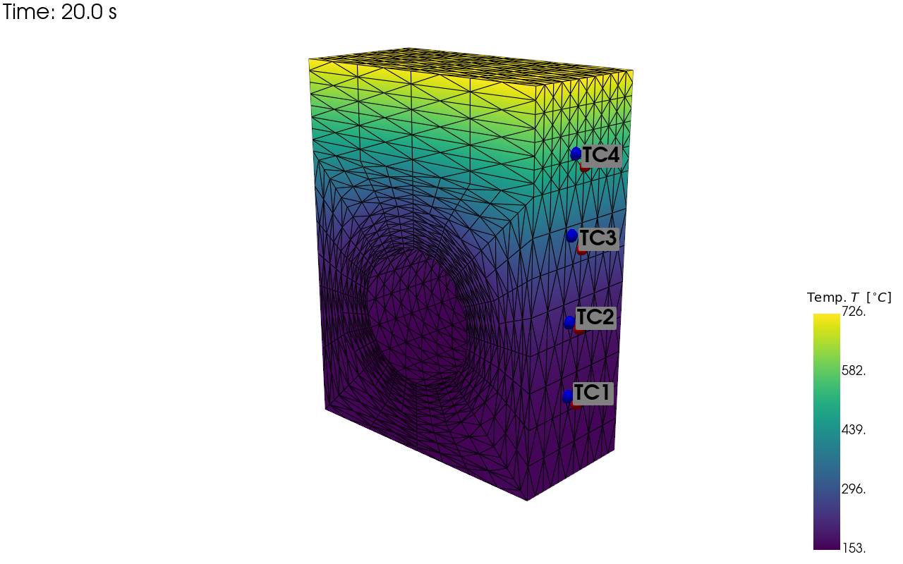
pv_plot = sens.plot_point_sensors_on_sim(sens_array,
                                         comp_key="temperature")

pv_plot.camera_position = [(59.354, 43.428, 69.946),
                           (-2.858, 13.189, 4.523),
                           (-0.215, 0.948, -0.233)]

# Set to False to show an interactive plot instead of saving the figure
pv_plot.off_screen = True
if pv_plot.off_screen:
    pv_plot.screenshot(output_path/"ext_ex4b_locs.png")
else:
    pv_plot.show()

Visualisation of nominal and perturbed sensor locations including the field errors.

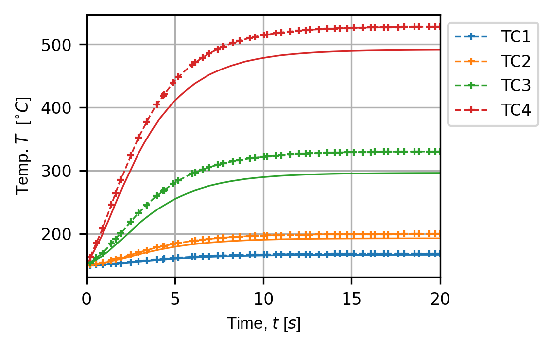
(fig,ax) = sens.plot_time_traces(sens_array,comp_key="temperature")
fig.savefig(output_path/"ext_ex4b_traces.png",dpi=300,bbox_inches="tight")

# Uncomment this to display the sensor trace plot
# plt.show()

Sensor traces showing the effects of the field error perturbing sensor location and sensor sample times.