Errors: basics

In this example we will provide an overview of the basic error library in pyvale. In pyvale errors have a type (random/systematic) and a dependence (independent/dependent). We can get an errors type using the .get_error_type() method returning an EErrType enumeration. We can also specify an errors dependence with the .set_error_dep() method and an EErrDep enumeration. If we recall the pyvale measurement simulation model:

measurement = truth + systematic errors + random errors

where all of these variables are numpy arrays with shape=(num_sensors, num_field_components,num_sample_times). This means an errors type will determine if it will be summed in the systematic on random error array.

The error dependence determines if an error is calculated based on the truth (independent) or the accumulated measurement based on all previous errors in the error chain (dependent). Some errors are purely independent such as random noise with a normal distribution with a set standard deviation. An example of an error that is dependent would be saturation which must be placed last in the error chain and will clamp the final sensor value to be within the specified bounds. We could also set any of the ‘percent’ errors to be dependent in which case the percentage would be calculated based on the accumulated sensor measurement at that point in the error chain instead of based on ground truth.

pyvale provides a library of different random ErrRand* and systematic ErrSys* errors which can be found listed in the docs. In the next example we will explore the more detailed parts of the error simulation library but for now we will specify some common error types. Try experimenting with the code below to turn the different error types off and on to see how it changes the virtual sensor measurements.

Note

It is also possible to write custom errors by writing your own class that implements the IErrSimulator abstract base class and then add them to your error chain. See the python API docs for IErrSimulator.

from pathlib import Path
import numpy as np
import matplotlib.pyplot as plt

# pyvale imports
import pyvale.mooseherder as mh
import pyvale.sensorsim as sens
import pyvale.dataset as dataset

1. Load physics simulation data

data_path: Path = dataset.thermal_3d_path()
sim_data: mh.SimData = mh.ExodusLoader(data_path).load_all_sim_data()
sim_data: mh.SimData = sens.scale_length_units(scale=1000.0,
                                               sim_data=sim_data,
                                               disp_keys=None)

2. Build virtual sensor array

sim_dims = sens.simtools.get_sim_dims(sim_data)
sens_pos: np.ndarray = sens.gen_pos_grid_inside(num_sensors=(1,4,1),
                                                x_lims=(12.5,12.5),
                                                y_lims=sim_dims["y"],
                                                z_lims=sim_dims["z"])

sample_times = np.linspace(0.0,np.max(sim_data.time),50)

sens_data = sens.SensorData(positions=sens_pos,
                            sample_times=sample_times)

sens_array: sens.SensorsPoint = sens.SensorFactory.scalar_point(
    sim_data,
    sens_data,
    comp_key="temperature",
    spatial_dims=sens.EDim.THREED,
    descriptor=sens.DescriptorFactory.temperature(),
)

2.1. Add simulated measurement errors

Now we have our sensor array applied to our simulation without any errors we can build a custom chain of basic errors. Here we will start by adding a series of systematic errors that are independent:

err_chain: list[sens.IErrSimulator] = []

For probability sampling systematic errors the distribution is sampled to provide an offset which is assumed to be constant over all sensor sampling times. This is different to random errors which are sampled to provide a different error for each sensor and time step.

These systematic errors provide a constant offset to all measurements in simulation units or as a percentage of the truth.

err_chain.append(sens.ErrSysOffset(offset=-10.0))
err_chain.append(sens.ErrSysOffsetPercent(offset_percent=-1.0))

pyvale includes a series of random number generator objects that wrap the random number generators from numpy. These are named Gen* and can be used with any of the ErrSysGen, ErrSysGenPercent, ErrRandGen or ErrRandGenPercent objects to create custom probability distribution sampling errors:

err_chain.append(sens.ErrSysGen(sens.GenUniform(low=-1.0,high=1.0)))
err_chain.append(sens.ErrSysGenPercent(sens.GenUniform(low=-1.0,high=1.0)))
err_chain.append(sens.ErrSysGen(sens.GenNormal(std=1.0)))
err_chain.append(sens.ErrSysGenPercent(sens.GenNormal(std=1.0)))
err_chain.append(
    sens.ErrSysGen(sens.GenTriangular(left=-1.0,mode=0.0,right=1.0))
)

We can also add a series of random errors in a similar manner to the systematic errors above noting that these will generate a new error for each sensor and each time step whereas the systematic error sampling provides a constant shift over all sampling times for each sensor.

err_chain.append(sens.ErrRandGen(sens.GenNormal(std=2.0)))
err_chain.append(sens.ErrRandGenPercent(sens.GenNormal(std=2.0)))
err_chain.append(sens.ErrRandGen(sens.GenUniform(low=-2.0,high=2.0)))
err_chain.append(sens.ErrRandGenPercent(sens.GenUniform(low=-2.0,high=2.0)))
err_chain.append(
    sens.ErrRandGen(sens.GenTriangular(left=-5.0,mode=0.0,right=5.0))
)

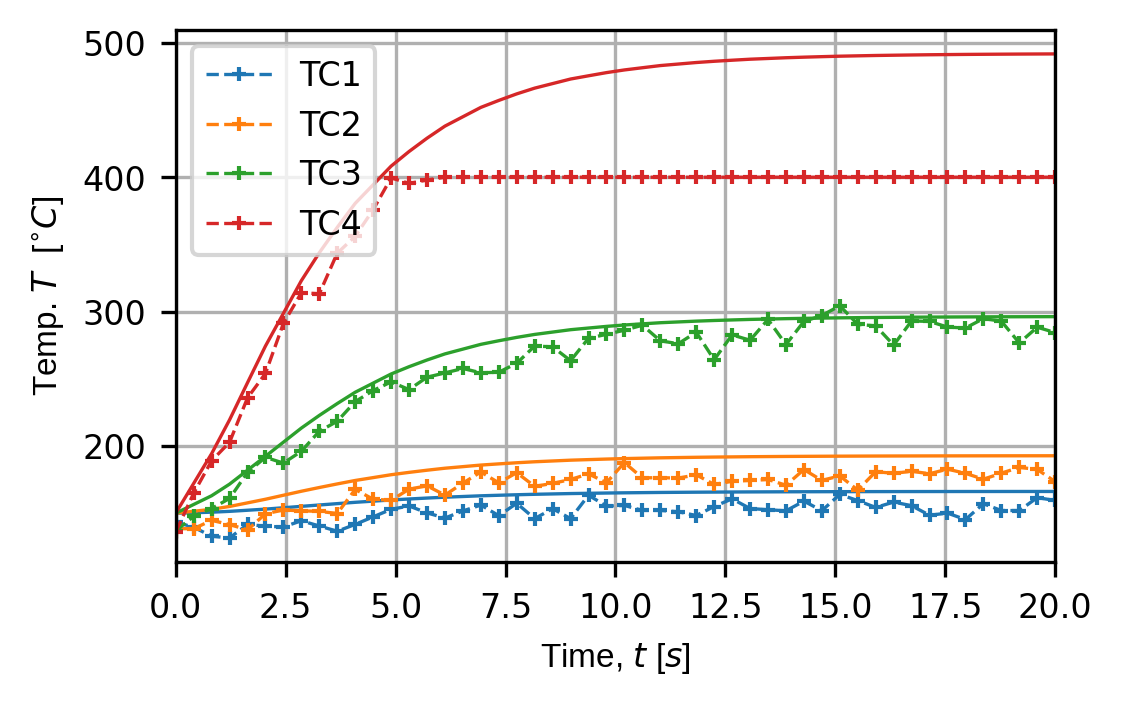
Finally, we add some dependent systematic errors including rounding errors, digitisation and saturation. Note that the saturation error must be placed last in the error chain. Try changing some of these values to see how the sensor traces change - particularly the saturation error.

err_chain.append(sens.ErrSysRoundOff(sens.ERoundMethod.ROUND,0.1))
err_chain.append(sens.ErrSysDigitisation(bits_per_unit=2**16/100))
err_chain.append(sens.ErrSysSaturation(meas_min=0.0,meas_max=400.0))

sens_array.set_error_chain(err_chain)

3. Run simulated experiment

measurements: np.ndarray = sens_array.sim_measurements()

truth: np.ndarray = sens_array.get_truth()
sys_errs: np.ndarray = sens_array.get_errors_systematic()
rand_errs: np.ndarray = sens_array.get_errors_random()

print(80*"-")
print("measurement = truth + sysematic error + random error")

print(f"measurements.shape = {measurements.shape} = "
        + "(n_sensors,n_field_components,n_timesteps)")
print(f"truth.shape     = {truth.shape}")
print(f"sys_errs.shape  = {sys_errs.shape}")
print(f"rand_errs.shape = {rand_errs.shape}")

sens_print: int = 3
comp_print: int = 0
time_last: int = 5
time_print = slice(measurements.shape[2]-time_last,measurements.shape[2])

print(f"\nThese are the last {time_last} virtual measurements of sensor "
        + f"{sens_print}:\n")

sens.print_measurements(sens_array,sens_print,comp_print,time_print)
print("\n"+80*"-")

4. Analyse & visualise the results

output_path = Path.cwd() / "pyvale-output"
if not output_path.is_dir():
    output_path.mkdir(parents=True, exist_ok=True)

(fig,ax) = sens.plot_time_traces(sens_array,comp_key="temperature")
fig.savefig(output_path/"ext_ex4a_traces.png",dpi=300,bbox_inches="tight")

# Uncomment this to display the sensor trace plot
# plt.show()