DIC with images generated from a virtual blender experiment

This example looks at taking the virtual experiments conducted using the blender module and taking it one step further and performing a DIC calculation on the simulated data. For this to work, you’ll need to complete the 2D image deformation example using the blender module first.

We’d recommend downloading both examples (links can be found at the bottom of each example) and placing them within the same folder on your device. That way the relative file paths below will not need to be changed.

import matplotlib.pyplot as plt
from pathlib import Path
import numpy as np
import os

# Pyvale imports
import pyvale.dic as dic

#subset size
subset_size = 21

# rename the reference image so that that we can distinguish between reference
# and deformed images
if os.path.exists("./blenderimages/blenderimage_0.tiff"):
    os.rename("./blenderimages/blenderimage_0.tiff",
              "./blenderimages/reference.tiff")

ref_img = "./blenderimages/reference.tiff"
def_img = "./blenderimages/blenderimage_*.tiff"

# Interactive ROI selection
roi = dic.RegionOfInterest(ref_img)
roi.interactive_selection(subset_size)

#output_path
output_path = Path.cwd() / "pyvale-output"
if not output_path.is_dir():
    output_path.mkdir(parents=True, exist_ok=True)

# DIC Calculation
dic.two_dimensional(reference=ref_img,
                           deformed=def_img,
                           roi_mask=roi.mask,
                           seed=roi.seed,
                           subset_size=subset_size,
                           subset_step=10,
                           shape_function="AFFINE",
                           max_displacement=20,
                           correlation_criteria="ZNSSD",
                           output_basepath=output_path,
                           output_prefix="blender_dic_")

# Import the Results
data_path = output_path / "blender_dic_*.csv"
dicdata = dic.data_import(data=data_path, delimiter=",",
                                 layout='matrix', binary=False)

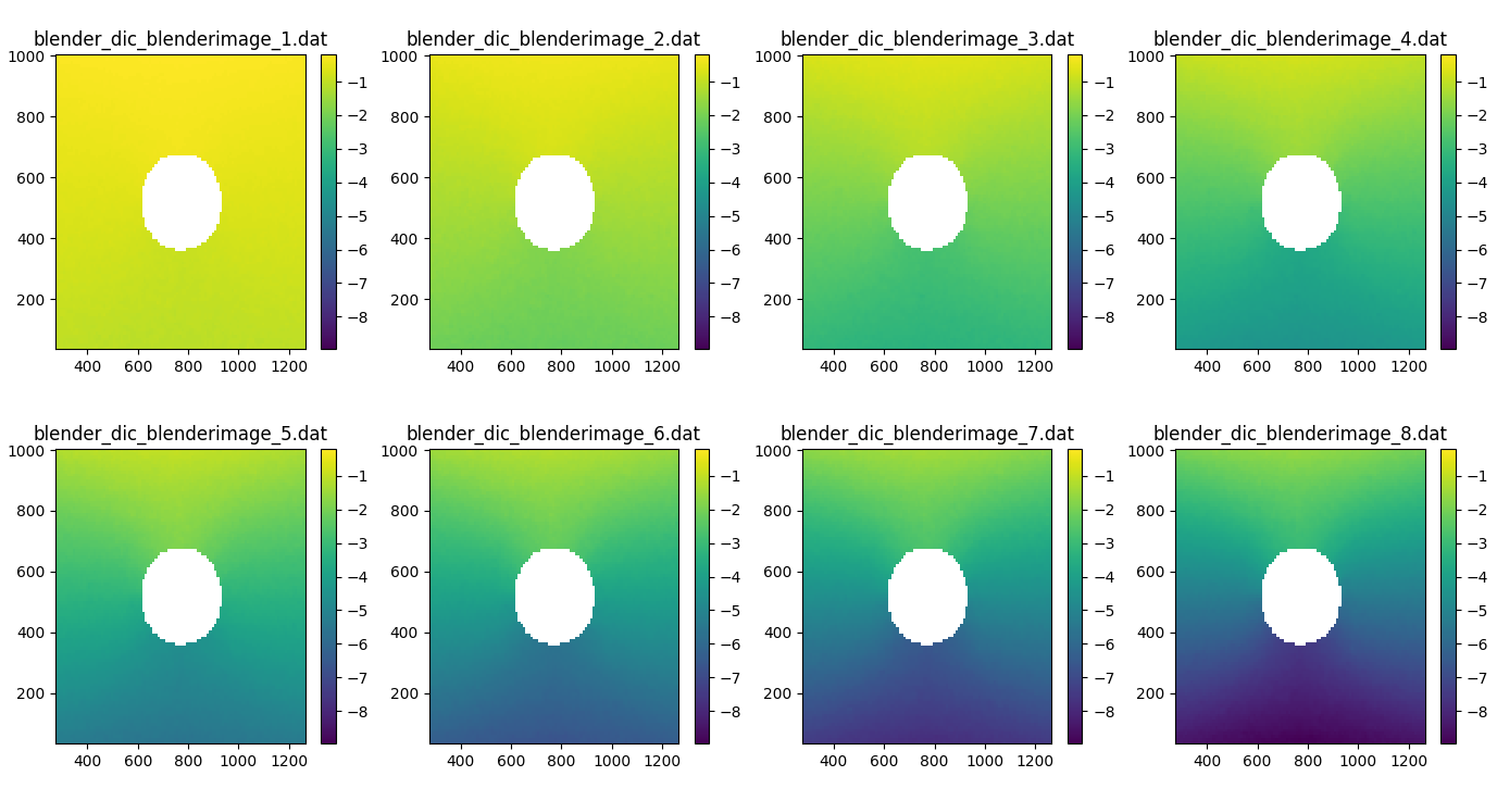
As an example we can plot the v-component of displacement for each of the eight deformation images

# Setup plot
fig, axes = plt.subplots(2, 4, figsize=(15, 5))
axes = axes.flatten()

# Compute global min and max for consistent color scaling
vmin = np.nanmin(dicdata.v)
vmax = np.nanmax(dicdata.v)
print(vmin,vmax)

# loop over images and add to subplots
for i in range(len(dicdata.filenames)):
    im = axes[i].pcolor(dicdata.ss_x, dicdata.ss_y, dicdata.v[i], vmin=vmin, vmax=vmax)
    axes[i].set_title(dicdata.filenames[i])
    fig.colorbar(im, ax=axes[i])

plt.tight_layout()
plt.show()