Scalar field sensor sim

In this example we introduce the basic features of pyvale for scalar field sensor simulation. We demonstrate quick sensor array construction with defaults using the pyvale sensor factory. We also introduce some key concepts for pyvale sensor simulation including error chains and the functions for running simulated sensor measurements as well as the data structures they are stored in. Finally, we run a sensor simulation, visualise the virtual sensor locations and plot the simulated sensor traces.

Before we begin the example, we will briefly describe the pyvale sensor measurement simulation model. In pyvale a simulated measurement is given by:

measurement = truth + systematic errors + random errors

The truth is interpolated from the input physics simulation to the virtual sensor positions and times. The systematic and random errors are evaluated for each masurement simulation by sampling probability distributions in a sequence called an error chain.

pyvale provides a library of common systematic (position uncertainty, spatial/temporal averaging, digitisation, calibration, etc.) and random errors (probability distribution in absolute units or as a percentage of the truth etc.). These errors all implement the IErrSimulator interface allowing a user to plug-and-play any combination of simulated errors in their error chain.

Ok, now let’s simulate some temperature measurements!

from pathlib import Path
import numpy as np
import matplotlib.pyplot as plt

# pyvale imports
import pyvale.sensorsim as sens
import pyvale.mooseherder as mh
import pyvale.dataset as dataset

1. Load physics simulation data

Here we load a MOOSE finite element simulation dataset that comes packaged with pyvale in exodus (*.e) format. pyvale loads simulations into a SimData object which contains the nodal coordinates, simulation time steps, the nodal physics variables and optionally the element connectivity tables.

We also convert the length units of our simulation from meters to milli-meters as our visualisation tools are based on unit scaling by default.

data_path: Path = dataset.thermal_3d_path()
sim_data: mh.SimData = mh.ExodusLoader(data_path).load_all_sim_data()

sim_data: mh.SimData = sens.scale_length_units(scale=1000.0,
                                               sim_data=sim_data,
                                               disp_keys=None)

Note

You can load your own exodus (*.e) file here by changing the path or you can load your own simulation data from delimited plain text files or numpy npy files. See the advanced example ‘Bring your own simulation data’.

2. Build virtual sensor arrays

First, we need to specify the position of our virtual sensors and the times that they should take simulated measurements as a numpy array. pyvale has helper functions for common sensor patterns like a regular grid inside given bounds but we could also have manually built the numpy array of sensor locations which has shape=(num_sensors,coord[x,y,z]).

The SensorData object allows us to specify the parameters to create the virtual sensor array. You can also set sample_times=None in SensorData which will make our virtual sensors sample at the simulation time steps.

sens_pos: np.ndarray = sens.gen_pos_grid_inside(num_sensors=(1,4,1),
                                                x_lims=(12.5,12.5),
                                                y_lims=(0.0,33.0),
                                                z_lims=(0.0,12.0))

sample_times: np.ndarray = np.linspace(0.0,np.max(sim_data.time),50)

sens_data = sens.SensorData(positions=sens_pos,
                            sample_times=sample_times)

We now create our virtual sensor array for a scalar field. We need to specify the component string key to be the same as for the nodal field variable we want our sensors to sample from in the SimData object. Our simulation is 3D so we specify that here and we add a descriptor (optional) that will be used to set the axes labels, symbols and units on our visualisations.

sens_array: sens.SensorsPoint = sens.SensorFactory.scalar_point(
    sim_data,
    sens_data,
    comp_key="temperature",
    spatial_dims=sens.EDim.THREED,
    descriptor=sens.DescriptorFactory.temperature(),
)

2.1. Add simulated measurement errors

Now we add some simulated errors to our sensor array with an error_chain which is a list of objects that implement the IErrSimulator interface. pyvale will evaluate these errors in the order they are specified in the list when we simulate our measurements. The error chain is the core of the pyvale sensor simulation engine.

err_chain: list[sens.IErrSimulator] = [
    sens.ErrSysGen(sens.GenUniform(low=-10.0,high=10.0)),
    sens.ErrRandGen(sens.GenNormal(std=5.0)),
]

sens_array.set_error_chain(err_chain)

3. Run a simulated experiment

We have built our sensor array so now we can call .sim_measurements() to generate simulated sensor traces. When we call this function pyvale will calculate the ground truth (if not already complete from a previous sim), then step through the error chain sampling probability distributions for our errors.

If we call .sim_measurements() again the process is repeated and the errors are resampled. However, if we call .get_measurements() then we are returned the previously simulated values. Throughout pyvale methods prefixed with get can be expected to return previous values if they exist whereas sim or `calc `methods will actually perform a simulation or calculation.

measurements: np.ndarray = sens_array.sim_measurements()

truth: np.ndarray = sens_array.get_truth()
sys_errs: np.ndarray = sens_array.get_errors_systematic()
rand_errs: np.ndarray = sens_array.get_errors_random()

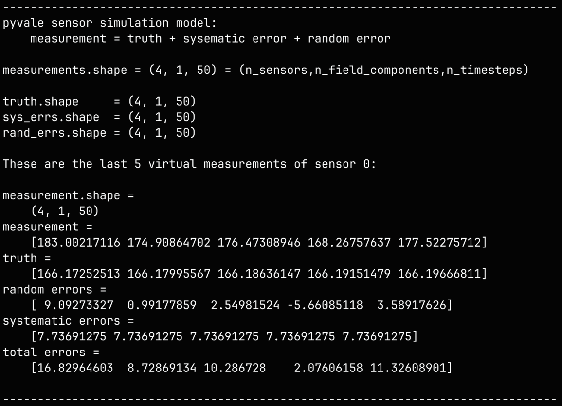
print(80*"-")
print("pyvale sensor simulation model:")
print("    measurement = truth + sysematic error + random error\n")

print(f"measurements.shape = {measurements.shape} = "
        + "(n_sensors,n_field_components,n_timesteps)\n")
print(f"truth.shape     = {truth.shape}")
print(f"sys_errs.shape  = {sys_errs.shape}")
print(f"rand_errs.shape = {rand_errs.shape}")

sens_print: int = 0
comp_print: int = 0
time_last: int = 5
time_print = slice(measurements.shape[2]-time_last,measurements.shape[2])

print(f"\nThese are the last {time_last} virtual measurements of sensor "
        + f"{sens_print}:\n")

sens.print_measurements(sens_array,sens_print,comp_print,time_print)
print("\n"+80*"-")

4. Analyse & visualise the results

We can now visualise the sensor locations on the simulation mesh and the simulated sensor traces using pyvale visualisation tools which are built on pyvista for meshes and matplotlib for sensor traces. pyvale will return figure and axes objects to the user allowing additional customisation using pyvista and matplotlib. This also means that we need to call .show() ourselves to display the figure as pyvale does not do this for us.

First we create our standard ‘pyvale-output’ directory to save images of our results to.

output_path = Path.cwd() / "pyvale-output"
if not output_path.is_dir():
    output_path.mkdir(parents=True, exist_ok=True)

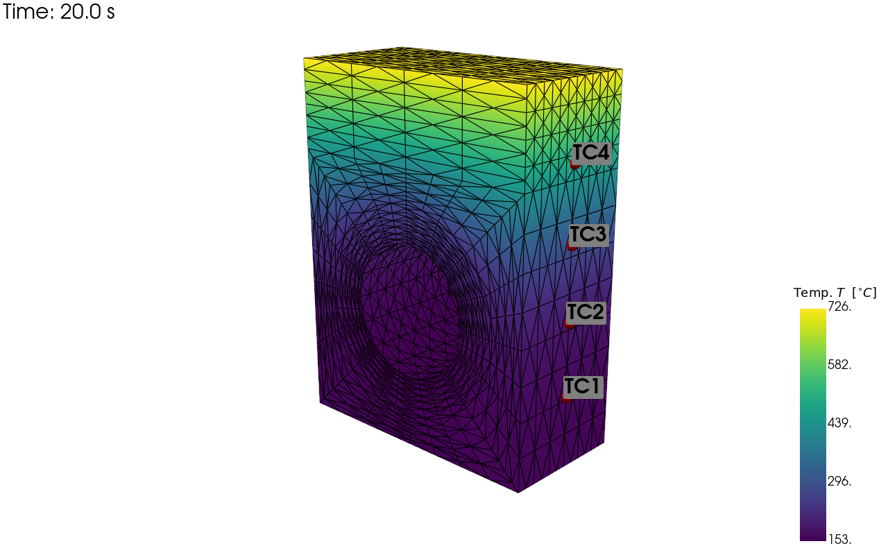
This creates a visualisation of our virtual sensor locations on the simulation mesh.

pv_plot = sens.plot_point_sensors_on_sim(sens_array,
                                         comp_key="temperature")

# Camera position determined in interactive mode and printed to terminal
# print(f"{pv_plot.camera_position=}")
pv_plot.camera_position = [(59.354, 43.428, 69.946),
                           (-2.858, 13.189, 4.523),
                           (-0.215, 0.948, -0.233)]


save_render: Path = output_path / "basics_ex1_locs.png"

# Set to False to show an interactive plot instead of saving the figure
pv_plot.off_screen = True
if pv_plot.off_screen:
    pv_plot.screenshot(save_render)

    # Uncomment to save a vector graphic
    # pv_plot.save_graphic(save_render.with_suffix(".svg"))
else:
    pv_plot.show()

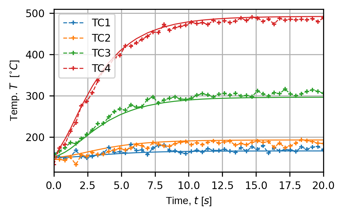
This creates a plot of the time traces for all of our sensors. The solid line shows the ‘truth’ and the dashed line with markers shows the simulated sensor traces. In other examples we will see how to configure this plot but for now we note we that we are returned a matplotlib figure and axes object which allows for further customisation.

(fig,ax) = sens.plot_time_traces(sens_array,comp_key="temperature")

save_traces = output_path/"basics_ex1_traces.png"
fig.savefig(save_traces, dpi=300, bbox_inches="tight")

# Uncomment this to display the sensor trace plot
# plt.show()