Vector and tensor field sensors

In this example we will show how pyvale can be used to simulate vector and tensor field sensors demonstrated by displacement and strain sensors. We show some of the additional sensor array setup parameters such as the sensor orientation for vector and tensor sensors. We also introduce a new type of simulated error called a ‘field error’ which can be used to simulate uncertainty in sensor positions, sampling time, orientation and sensor averaging area.

from pathlib import Path
import numpy as np
from scipy.spatial.transform import Rotation
import matplotlib.pyplot as plt

# pyvale imports
import pyvale.mooseherder as mh
import pyvale.sensorsim as sens
import pyvale.dataset as dataset

1. Load physics simulation data

As we did in the last example we load a finite element simulation dataset that comes packaged with pyvale in exodus (*.e) format. We also convert the length units of our simulation from meters to milli-meters as our visualisation tools are based on unit scaling by default.

data_path: Path = dataset.mechanical_2d_path()
sim_data: mh.SimData = mh.ExodusLoader(data_path).load_all_sim_data()

disp_keys = ("disp_x","disp_y")
strain_norm_keys = ("strain_xx","strain_yy",)
strain_dev_keys = ("strain_xy",)

sim_data: mh.SimData  = sens.scale_length_units(scale=1000.0,
                                                sim_data=sim_data,
                                                disp_keys=disp_keys)

2. Build virtual sensor arrays

Creating a vector or tensor field sensor array is similar to what we have already done for scalar fields we just need to specify the string keys for the field components we want to use in the sim data object we have loaded. For vector and tensor field sensors we can also specify a sensor orientation which we demonstrate here.

The information we provide in the SensorData object is treated as the ground truth so any ‘field errors’ we simulate later are calculated with respect to this.

sens_pos: np.ndarray = sens.gen_pos_grid_inside(num_sensors=(2,2,1),
                                                x_lims=(0.0,100.0),
                                                y_lims=(0.0,150.0),
                                                z_lims=(0.0,0.0))

sample_times: np.ndarray = np.linspace(0.0,np.max(sim_data.time),50)

sens_angles: tuple[Rotation] = sens_pos.shape[0] * \
    (Rotation.from_euler("zyx",[90,0,0], degrees=True),)

disp_sens_data = sens.SensorData(positions=sens_pos,
                                 sample_times=sample_times,
                                 angles=sens_angles)

disp_sens: sens.SensorsPoint = sens.SensorFactory.vector_point(
    sim_data,
    disp_sens_data,
    comp_keys=disp_keys,
    spatial_dims=sens.EDim.TWOD,
    descriptor=sens.DescriptorFactory.displacement(),
)

Note

Sensor angles can be specified individually for all sensors or if all sensors have the same angle a single element tuple can be used. This has the advantage that the rotations can be batch executed in one numpy call for speed. So we could have used sens_angles = (Rotation.from_euler(“zyx”, [90,0,0],degrees=True),) above.

For the tensor field sensors we have to separately specify the string keys for the normal and deviatoric tensor components, otherwise it is the same as for the vector field sensor.

strain_sens_data = sens.SensorData(positions=sens_pos,
                                   sample_times=sample_times,
                                   angles=sens_angles)

strain_sens: sens.SensorsPoint = sens.SensorFactory.tensor_point(
    sim_data,
    strain_sens_data,
    norm_comp_keys=strain_norm_keys,
    dev_comp_keys=strain_dev_keys,
    spatial_dims=sens.EDim.TWOD,
    descriptor=sens.DescriptorFactory.strain(sens.EDim.TWOD),
)

2.1. Add simulated measurement errors

Now we are going to create an error that allows us to add uncertainty in the sensor position and angle (as well as the sampling time and area averaging). In pyvale these are called field errors because we have to re-interpolate the field to evaluate them. In this case we will have a constant offset and random perturbation in the sensor positions and angle. We use the same type of field error for both sensor arrays for simplicity and add a probabilistic random error.

First, we setup the data structures that will tell our error chain how to configure and evaluate our field errors. Everything that can be evaluated in a field error is captured in the ErrFieldData dataclass.

pos_offset_xyz = np.array((2.0,2.0,0.0),dtype=np.float64)
pos_offset_xyz = np.tile(pos_offset_xyz,(sens_pos.shape[0],1))

pos_rand = sens.GenUniform(low=-2.0,high=2.0)  # units = mm

angle_offset = np.zeros_like(sens_pos)
angle_offset[:,0] = 1.0 # only rotate about z in 2D, units = degrees

angle_rand = sens.GenUniform(low=-5.0,high=5.0)

field_err_data = sens.ErrFieldData(pos_offset_xyz=pos_offset_xyz,
                                   pos_rand_xyz=(pos_rand,pos_rand,None),
                                   ang_offset_zyx=angle_offset,
                                   ang_rand_zyx=(angle_rand,None,None))

We build and set our error chains in exactly the same way as we did before noting that our field errors need a reference to the field that they will have to interpolate.

disp_err_chain: list[sens.IErrSimulator] = [
    sens.ErrRandGen(sens.GenNormal(std=2.0)),
    sens.ErrSysField(disp_sens.get_field(),field_err_data),
]

disp_sens.set_error_chain(disp_err_chain)

strain_err_chain: list[sens.IErrSimulator] = [
    sens.ErrRandGenPercent(sens.GenUniform(low=-2.0,high=2.0)),
    sens.ErrSysField(strain_sens.get_field(),field_err_data),
]
strain_sens.set_error_chain(strain_err_chain)

3. Run a simulated experiment

We run our sensor simulation as normal but we note that the second dimension of our measurement array will have either 2 vector components for the displacement sensors in 2D or 3 tensor components for the strain sensors in 2D.

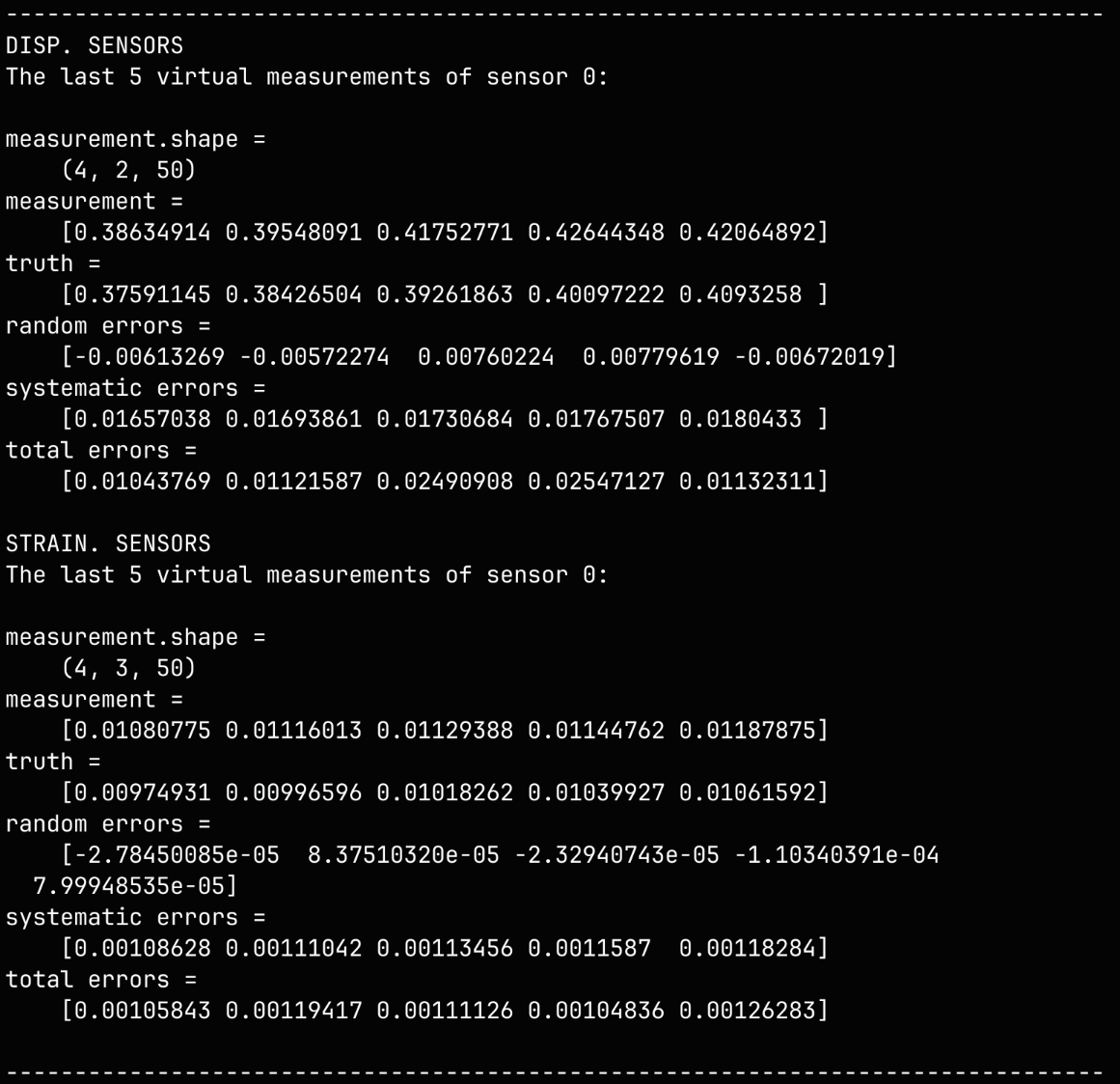
We also print some of the virtual displacement and strain measurements to the console along with the shapes of the measurement arrays so we can compare them. Note that for the tensor sensors the measurement array axis is ordered so that the normal components are followed by the deviatoric.

disp_meas: np.ndarray = disp_sens.sim_measurements()
strain_meas: np.ndarray = strain_sens.sim_measurements()

sens_print: int = 0
comp_print: int = 0
time_last: int = 5
time_print = slice(disp_meas.shape[2]-time_last,disp_meas.shape[2])

print(80*"-")
print("DISP. SENSORS")
print(f"The last {time_last} virtual measurements of sensor "
        + f"{sens_print}:\n")

sens.print_measurements(disp_sens,sens_print,comp_print,time_print)

print("\nSTRAIN. SENSORS")
print(f"The last {time_last} virtual measurements of sensor "
        + f"{sens_print}:\n")

sens.print_measurements(strain_sens,sens_print,comp_print,time_print)
print("\n"+80*"-")

Example terminal output:

4. Analyse & visualise the results

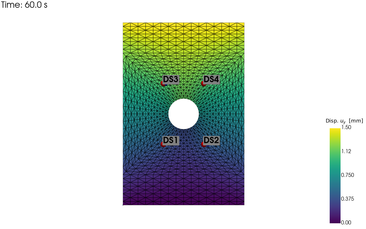
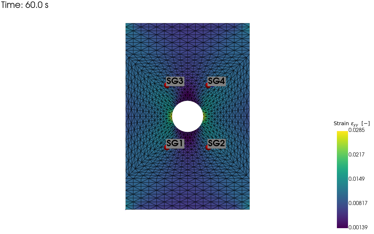
Now we visualise the sensor locations on the mesh and save these images to disk. As we have used sensor positioning errors in our error chain the perturbed sensor locations are shown on the sensor location visualisation as different coloured spheres without labels.

output_path = Path.cwd() / "pyvale-output"
if not output_path.is_dir():
    output_path.mkdir(parents=True, exist_ok=True)


pv_plot = sens.plot_point_sensors_on_sim(disp_sens,"disp_y")
pv_plot.camera_position = "xy"

save_render = output_path / "basics_ex2_disp_locs.png"

# Set to False to show an interactive plot instead of saving the figure
pv_plot.off_screen = True
if pv_plot.off_screen:
    pv_plot.screenshot(save_render)
else:
    pv_plot.show()

pv_plot = sens.plot_point_sensors_on_sim(strain_sens,"strain_yy")
pv_plot.camera_position = "xy"

# Set to False to show an interactive plot instead of saving the figure
pv_plot.off_screen = True
if pv_plot.off_screen:
    pv_plot.screenshot(output_path / "basics_ex2_strain_locs.png")
else:
    pv_plot.show()

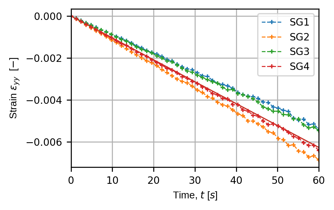
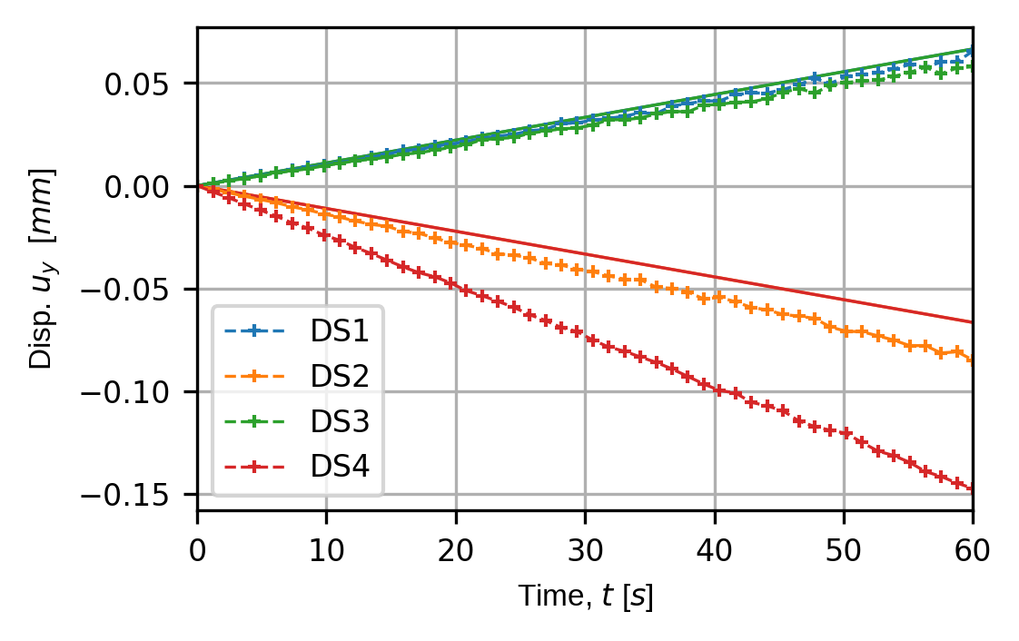
We also plot and save the time traces for our virtual sensors for all components of the displacement and strain fields and save them to disk.

for kk in disp_keys:
    (fig,ax) = sens.plot_time_traces(disp_sens,kk)

    save_traces = output_path/f"basics_ex2_traces_{kk}.png"
    fig.savefig(save_traces, dpi=300, bbox_inches="tight")

for kk in (strain_norm_keys+strain_dev_keys):
    (fig,ax) = sens.plot_time_traces(strain_sens,kk)

    save_traces = output_path/f"basics_ex2_traces_{kk}.png"
    fig.savefig(save_traces, dpi=300, bbox_inches="tight")

# Uncomment to show all traces plots
# plt.show()