Quickstart sensor sim

This is a quick example with minimal explanation to get users familiar with the overall workflow for the pyvale sensor simulation engine - to see if pyvale is the right virtual laboratory for them.

The general workflow for the sensor simulation engine in pyvale is: 1. Load physics simulation data; 2. Build virtual sensor arrays (with errors); 3. Create & run a simulated experiment; and 4. Analyse & visualise the results.

Users with experience in scientific and engineering simulation will recognise the workflow as: setup/pre-processing; run simulation; post-processing, analysis & visualisation.

from pathlib import Path
import numpy as np
import matplotlib.pyplot as plt

# pyvale imports
import pyvale.sensorsim as sens
import pyvale.mooseherder as mh
import pyvale.dataset as dataset

1. Load physics simulation data

data_path: Path = dataset.thermomechanical_3d_path()
sim_data: mh.SimData = mh.ExodusLoader(data_path).load_all_sim_data()
sim_data: mh.SimData = sens.scale_length_units(scale=1000.0,
                                               sim_data=sim_data,
                                               disp_keys=None)

2. Build a virtual sensor array

sens_pos: np.ndarray = sens.gen_pos_grid_inside(num_sensors=(1,4,1),
                                                    x_lims=(12.5,12.5),
                                                    y_lims=(0.0,33.0),
                                                    z_lims=(0.0,12.0))
sens_data = sens.SensorData(positions=sens_pos)

sens_array: sens.SensorsPoint = sens.SensorFactory.scalar_point(
    sim_data,
    sens_data,
    comp_key="temperature",
    spatial_dims=sens.EDim.THREED,
    descriptor=sens.DescriptorFactory.temperature(),
)

2.1. Add simulated measurement errors

err_chain: list[sens.IErrSimulator] = [
    sens.ErrSysGen(sens.GenUniform(low=-1.0,high=1.0)),
    sens.ErrSysGenPercent(sens.GenUniform(low=-1.0,high=1.0)),
    sens.ErrRandGen(sens.GenNormal(std=1.0)),
    sens.ErrRandGenPercent(sens.GenNormal(std=2.0)),
    sens.ErrSysDigitisation(bits_per_unit=2**16/100),
    sens.ErrSysSaturation(meas_min=0.0,meas_max=450.0),
]
sens_array.set_error_chain(err_chain)

3. Create & run simulated experiment

sims: dict[str,mh.SimData] = {"sim_nominal":sim_data,}
sensors: dict[str,sens.ISensorArray] = {"temp_sens":sens_array,}

exp_sim_opts = sens.ExpSimOpts(workers=4,para=sens.EExpSimPara.ALL)
exp_sim = sens.ExperimentSimulator(sims,sensors,exp_sim_opts)

exp_data: dict[tuple[str,...],np.ndarray] = (
    exp_sim.run_experiments(num_exp_per_sim=100)
)

exp_stats: dict[tuple[str,...],sens.ExpSimStats] = (
    sens.calc_exp_sim_stats(exp_data)
)

4. Analyse & visualise the results

output_path = Path.cwd() / "pyvale-output"
if not output_path.is_dir():
    output_path.mkdir(parents=True, exist_ok=True)

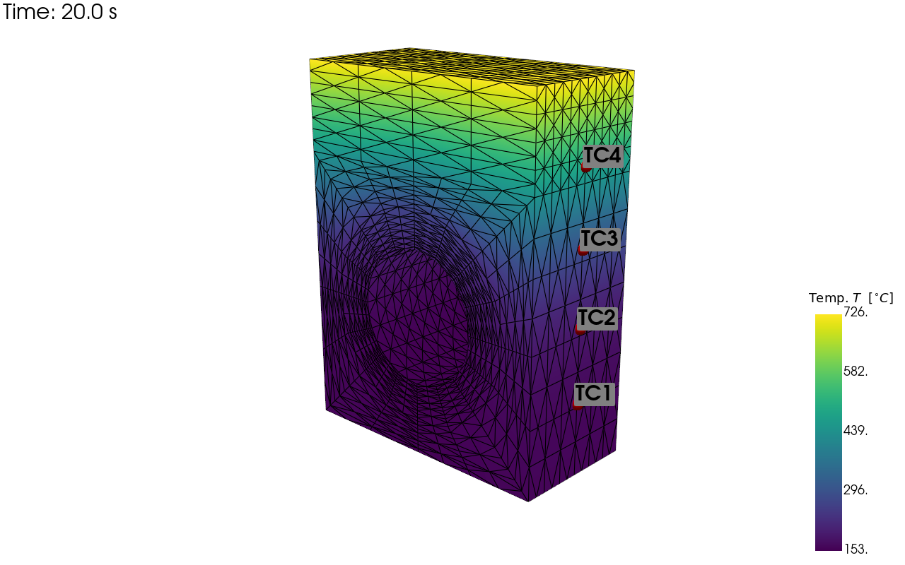
pv_plot = sens.plot_point_sensors_on_sim(sens_array,"temperature")
pv_plot.camera_position = [(59.354, 43.428, 69.946),
                            (-2.858, 13.189, 4.523),
                            (-0.215, 0.948, -0.233)]

# Set to False to show an interactive plot instead of saving the figure
pv_plot.off_screen = True
if pv_plot.off_screen:
    pv_plot.screenshot(output_path/"basics_ex0_locs.png")
else:
    pv_plot.show()

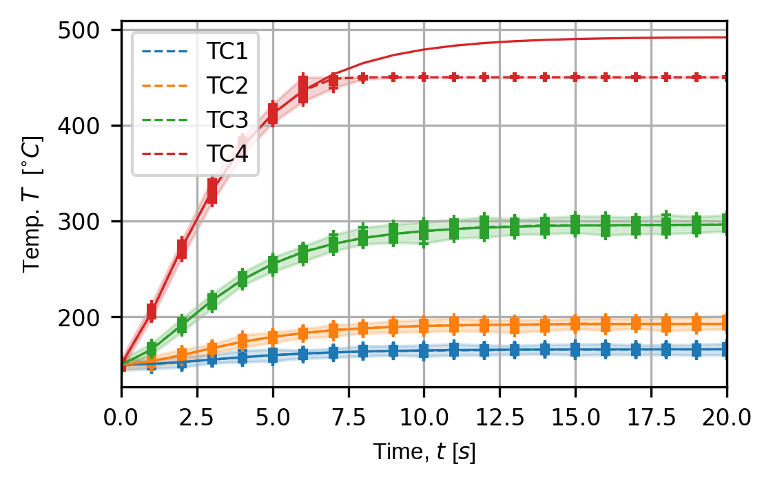
trace_opts = sens.TraceOptsExperiment(plot_all_exp_points=True)
(fig,ax) = sens.plot_exp_traces(
    exp_data,
    comp_ind=0,
    sens_key="temp_sens",
    sim_key="sim_nominal",
    descriptor=sens.DescriptorFactory.temperature(),
    trace_opts=trace_opts,
)

fig.savefig(output_path/"basics_ex0_traces.png",dpi=300,bbox_inches="tight")

# Uncomment to show interactive figure
# plt.show()