Errors: field-based chaining¶

In this example we show how field errors can be chained together and accumulated allowing for successive perturbations in position, sampling time and orientation. In order to do this we need to set our field error to be ‘dependent’. Note that it is more computationally efficient to provide a single field error object as this will perform all perturbations in a single step allowing for a single new interpolation of the underlying physical field. However, in some cases it can be useful to separate the sensor parameter perturbations to determine which is contributing most to the total error.

Under the hood the pyvale sensor simulation module uses and

from pathlib import Path
import numpy as np
from scipy.spatial.transform import Rotation
import matplotlib.pyplot as plt

# pyvale imports
import pyvale.mooseherder as mh
import pyvale.sensorsim as sens
import pyvale.dataset as dataset

1. Load physics simulation data¶

data_path: Path = dataset.mechanical_2d_path()
sim_data: mh.SimData = mh.ExodusLoader(data_path).load_all_sim_data()

disp_keys = ("disp_x","disp_y")
strain_norm_keys = ("strain_xx","strain_yy",)
strain_dev_keys = ("strain_xy",)

sim_data: mh.SimData  = sens.scale_length_units(scale=1000.0,
                                                sim_data=sim_data,
                                                disp_keys=disp_keys)

2. Build virtual sensor arrays¶

sim_dims: dict[str,tuple[float,float]] = sens.simtools.get_sim_dims(sim_data)
sens_pos: np.ndarray = sens.gen_pos_grid_inside(num_sensors=(2,2,1),
                                                x_lims=sim_dims["x"],
                                                y_lims=sim_dims["y"],
                                                z_lims=(0.0,0.0))

sample_times: np.ndarray = np.linspace(0.0,np.max(sim_data.time),50)

sens_angles: tuple[Rotation] = (
    Rotation.from_euler("zyx",[0,0,0], degrees=True),
)

sens_data = sens.SensorData(positions=sens_pos,
                            sample_times=sample_times,
                            angles=sens_angles)

sens_array: sens.SensorsPoint = sens.SensorFactory.vector_point(
    sim_data,
    sens_data,
    comp_keys=disp_keys,
    spatial_dims=sens.EDim.TWOD,
    descriptor=sens.DescriptorFactory.displacement(),
)

2.1. Add simulated measurement errors¶

Now we will build a series of field errors that cause successive offsets in sensor sampling time, sensor position and sensor orientation. That way we should be able to analyse the sensor data object at each point in the error chain to see how the sensor parameters have accumulated. We will apply a position offset of -1.0mm in the x and y axes.

pos_offset = -1.0*np.ones_like(sens_pos)
pos_offset[:,2] = 0.0 # in 2d we only have offset in x and y so zero z
pos_error_data = sens.ErrFieldData(pos_offset_xyz=pos_offset)

We will then apply a rotation offset about the z axis of 1 degree

angle_offset = np.zeros_like(sens_pos)
angle_offset[:,0] = 1.0 # only rotate about z in 2D
angle_error_data = sens.ErrFieldData(ang_offset_zyx=angle_offset)

time_offset = 2.0*np.ones_like(sens_array.get_sample_times())
time_error_data = sens.ErrFieldData(time_offset=time_offset)

Now we add all our field errors to our error chain. We add each error twice to see how they accumulate with each other. We explicitly set the error dependence to DEPENDENT so that the sensor state is accumulated over the error chain. Note that DEPENDENT is the default for field errors so that the perturbations to the sensor data are accumulated.

Instead of setting the dependence for each individual error above we could also just use our error integration options to force all errors to be DEPENDENT. We also set the error integration options to store the errors for each step in the error chain so we can analyse the sensor data at each step of chain. This option also allows us to separate the contribution of each error in the chain to the total error rather than just being able to analyse the total systematic and total random error which is the default. Note that this option will use more memory.

err_int_opts = sens.ErrIntOpts(force_dependence=sens.EErrDep.DEPENDENT,
                               store_all_errs=True)

sens_array.set_error_chain(err_chain,err_int_opts)

3. Create & run simulated experiment¶

Here we will print to the console the time, position and angle of from the sensor data objects at each point in the error chain. We should see each sensor parameter perturbed and accumulated throughout the chain.

measurements = sens_array.sim_measurements()

err_int = sens_array.get_error_integrator()

sens_data_by_chain = err_int.get_sens_data_by_chain()
if sens_data_by_chain is not None:
    for ii,ss in enumerate(sens_data_by_chain):
        print(80*"-")
        if ss is not None:
            print(f"SensorData @ [{ii}]")
            print("TIME")
            print(ss.sample_times)
            print()
            print("POSITIONS")
            print(ss.positions)
            print()
            print("ANGLES")
            for aa in ss.angles:
                print(aa.as_euler("zyx",degrees=True))
            print()
        print(80*"-")

Try setting all the field errors to be INDEPENDENT using the error integration options above. You should see that the sensor parameters are not accumulated throughout the error chain.

Wen ow print the results for one of the sensors so we can see what the errors are for the last few sampling times.

print(80*"-")

sens_print = 0
comp_print = 0
time_last = 5
time_print = slice(measurements.shape[2]-time_last,measurements.shape[2])

print("SENSORS WITH ACCUMULATED FIELD ERRORS:")
print(f"These are the last {time_last} virtual measurements of sensor "
        + f"{sens_print} for {disp_keys[comp_print]}:")

sens.print_measurements(sens_array,sens_print,comp_print,time_print)

print(80*"-")

4. Visualise the results¶

output_path = Path.cwd() / "pyvale-output"
if not output_path.is_dir():
    output_path.mkdir(parents=True, exist_ok=True)

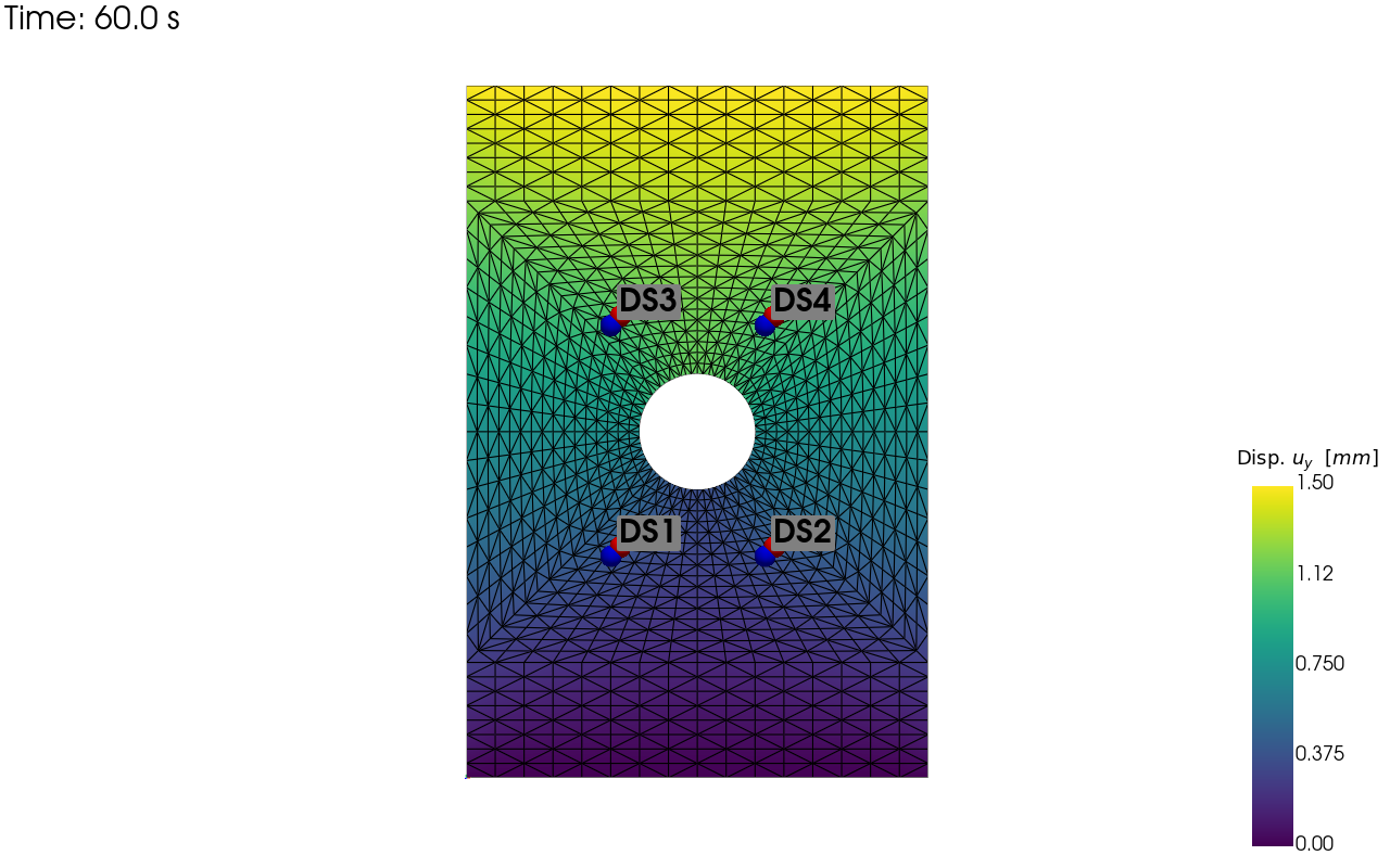
pv_plot = sens.plot_point_sensors_on_sim(sens_array,"disp_y")
pv_plot.camera_position = "xy"

save_render = output_path/"ext_ex4e_locs.png"

pv_plot.off_screen = True
if pv_plot.off_screen:
    pv_plot.screenshot(save_render)
else:
    pv_plot.show()

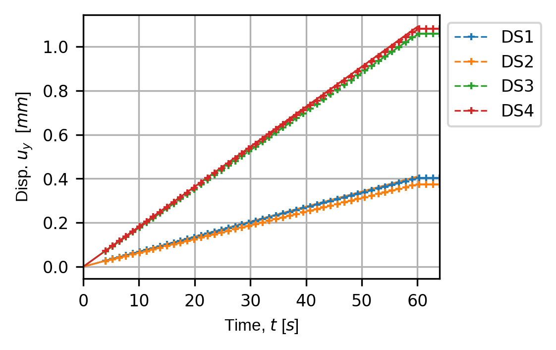
for kk in disp_keys:
    (fig,ax) = sens.plot_time_traces(sens_array,kk)
    save_traces = output_path/f"ext_ex4e_traces_{kk}.png"
    fig.savefig(save_traces, dpi=300, bbox_inches="tight")

# Uncomment this to display the sensor trace plot
# plt.show()

Gallery generated by Sphinx-Gallery