Experiment simulation in 3D

In this example we apply multiple sensor arrays across a number of different physics simulations with different inputs allowing us to run a series of virtual experiments and analyse the results.

Note that this example has minimal explanation and assumes you have reviewed the basic sensor simulation examples to understand how the underlying engine works as well as the sensor simulation workflow.

import time
from pathlib import Path
import numpy as np
import matplotlib.pyplot as plt

# pyvale imports
import pyvale.mooseherder as mh
import pyvale.sensorsim as sens
import pyvale.dataset as dataset

1. Load physics simulation data

sim_paths: list[Path] = dataset.thermomechanical_3d_experiment_paths()
sim_keys: set[str] = {"sim_nominal","sim_perturbed"}

disp_keys = ("disp_x","disp_y","disp_z")
strain_norm_keys = ("strain_xx","strain_yy","strain_zz")
strain_dev_keys = ("strain_xy","strain_yz","strain_xz")

sim_data_dict: dict[str,mh.SimData] = {}
for ss,kk in zip(sim_paths,sim_keys):
    sim_data: mh.SimData = mh.ExodusLoader(ss).load_all_sim_data()

    sim_data: mh.SimData = sens.scale_length_units(scale=1000.0,
                                                   sim_data=sim_data,
                                                   disp_keys=disp_keys)
    sim_data_dict[kk] = sim_data

2. Build virtual sensor arrays

2.1 Build scalar field sensor array

sample_times = np.linspace(0.0,np.max(sim_data.time),50)

temp_sens_pos: np.ndarray = sens.gen_pos_grid_inside(num_sensors=(1,4,1),
                                                     x_lims=(12.5,12.5),
                                                     y_lims=(0.0,33.0),
                                                     z_lims=(0.0,12.0))

temp_sens_data = sens.SensorData(positions=temp_sens_pos,
                                 sample_times=sample_times)

temp_sens: sens.SensorsPoint = sens.SensorFactory.scalar_point(
    sim_data,
    temp_sens_data,
    comp_key="temperature",
    spatial_dims=sens.EDim.THREED,
    descriptor=sens.DescriptorFactory.temperature(),
)

2.2 Add errors to the scalar field sensors

temp_pos_uncert = 0.25 # units = mm
temp_pos_rand = (None,
                 sens.GenNormal(std=temp_pos_uncert),
                 sens.GenNormal(std=temp_pos_uncert))

temp_field_err_data = sens.ErrFieldData(pos_rand_xyz=temp_pos_rand)

temp_err_chain: list[sens.IErrSimulator] = [
    sens.ErrSysField(temp_sens.get_field(),temp_field_err_data),
    sens.ErrRandGen(sens.GenNormal(std=2.0)), # units = degrees
    sens.ErrSysDigitisation(bits_per_unit=2**24/100),
    sens.ErrSysSaturation(meas_min=0.0,meas_max=700.0),
]

temp_sens.set_error_chain(temp_err_chain)

2.3 Build tensor field sensor array

strain_sens_pos: np.ndarray = sens.gen_pos_grid_inside(num_sensors=(1,4,1),
                                                       x_lims=(9.4,9.4),
                                                       y_lims=(0.0,33.0),
                                                       z_lims=(12.0,12.0))

strain_sens_data = sens.SensorData(positions=strain_sens_pos,
                                   sample_times=sample_times)

strain_sens: sens.SensorsPoint = sens.SensorFactory.tensor_point(
    sim_data,
    strain_sens_data,
    norm_comp_keys=strain_norm_keys,
    dev_comp_keys=strain_dev_keys,
    spatial_dims=sens.EDim.THREED,
    descriptor=sens.DescriptorFactory.strain(sens.EDim.THREED),
)

2.4 Add errors to the tensor field sensors

strain_max: float = 5000.0e-6 # 5000 micro-strain max before sensor fails

strain_pos_uncert: float = 0.25
strain_pos_rand_xyz = (
    sens.GenUniform(low=-strain_pos_uncert,high=strain_pos_uncert),
    sens.GenUniform(low=-strain_pos_uncert,high=strain_pos_uncert),
    None,
)

strain_angle_uncert: float = 1.0 # units = degrees
strain_angle_rand_zyx = (
    sens.GenUniform(low=-strain_angle_uncert,high=strain_angle_uncert),
    None,
    None,
)

strain_field_err_data = sens.ErrFieldData(pos_rand_xyz=strain_pos_rand_xyz,
                                          ang_rand_zyx=strain_angle_rand_zyx)

strain_err_chain: list[sens.IErrSimulator] = [
    sens.ErrSysField(strain_sens.get_field(),strain_field_err_data),
    sens.ErrRandGenPercent(sens.GenNormal(std=2.0)),
    sens.ErrSysDigitisation(bits_per_unit=2**24/strain_max),
    sens.ErrSysSaturation(meas_min=-strain_max,meas_max=strain_max),
]
strain_sens.set_error_chain(strain_err_chain)

3. Create & run simulated experiments

sensor_arrays: dict[str,sens.ISensorArray] = {
    "temp": temp_sens,
    "strain": strain_sens,
}

exp_sim_opts = sens.ExpSimOpts(workers=4,para=sens.EExpSimPara.ALL)
exp_save_keys = sens.ExpSimSaveKeys(pert_sens_times=None)

exp_sim = sens.ExperimentSimulator(sim_data_dict,
                                   sensor_arrays,
                                   exp_sim_opts,
                                   exp_save_keys)

start_exp: float = time.perf_counter()
exp_data: dict[tuple[str,...],np.ndarray] = (
    exp_sim.run_experiments(num_exp_per_sim=1000)
)
exp_time: float = time.perf_counter() - start_exp

start_stats: float = time.perf_counter()
exp_stats: dict[tuple[str,...],sens.ExpSimStats] = (
    sens.calc_exp_sim_stats(exp_data)
)
stats_time: float = time.perf_counter() - start_stats

print(80*"-")
print(f"Exp. sim. time    = {exp_time:.3f} seconds")
print(f"Stats. calc. time = {stats_time:.3f} seconds")
print(80*"-")
print()

4. Analyse & visualise the results

print(80*"-")
print("Keys in the simulated experimental data dictionary:")
for kk in exp_data:
    print(kk)
print(80*"-")
print()

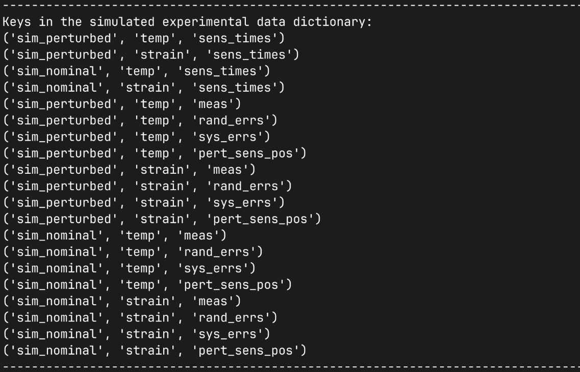
print(80*"-")
print("Thermal sensor array:")
print()
print(f"    {exp_data[('sim_nominal','temp','meas')].shape=}")
print("    shape=(n_exps,n_sensors,n_field_comps,n_time_steps)")
print()
print(f"    {exp_stats[('sim_nominal','temp','meas')].max.shape=}")
print("    shape=(n_sensors,n_field_comps,n_time_steps)")
print()
print(f"    {exp_data[('sim_nominal','temp','pert_sens_pos')].shape=}")
print("    shape=(n_exps,n_sensors,coord[X,Y,Z])")
print()
print(80*"-")
print("Mechanical sensor array:")
print()
print(f"    {exp_data[('sim_nominal','strain','meas')].shape=}")
print("    shape=(n_exps,n_sensors,n_field_comps,n_time_steps)")
print()
print(f"    {exp_stats[('sim_nominal','strain','meas')].max.shape=}")
print("    shape=(n_sensors,n_field_comps,n_time_steps)")
print()
print(f"    {exp_data[('sim_nominal','strain','pert_sens_pos')].shape=}")
print("    shape=(n_exps,n_sensors,coord[X,Y,Z])")
print()
print(80*"-")

output_path: Path = Path.cwd() / "pyvale-output"
if not output_path.is_dir():
    output_path.mkdir(parents=True, exist_ok=True)

sens.save_exp_sim_data(output_path/"ex5b_exp_sim_data.npz",exp_data)


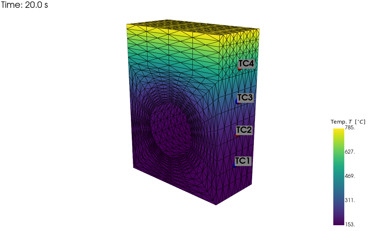
cam_pos = np.array([(59.354, 43.428, 69.946),
                    (-2.858, 13.189, 4.523),
                    (-0.215, 0.948, -0.233)])

pert_sens_pos = exp_data[("sim_nominal","temp","pert_sens_pos")][-1,:,:]
pv_plot = sens.plot_point_sensors_on_sim(sensor_array=temp_sens,
                                         comp_key="temperature",
                                         time_step=-1,
                                         perturbed_sens_pos=pert_sens_pos)
pv_plot.camera_position = cam_pos

# Set to False to show an interactive plot instead of saving the figure
pv_plot.off_screen = True
if pv_plot.off_screen:
    pv_plot.screenshot(output_path/"ext_ex5b_temp_locs.png")
else:
    pv_plot.show()

Visualisation of the virtual temperature sensor locations:

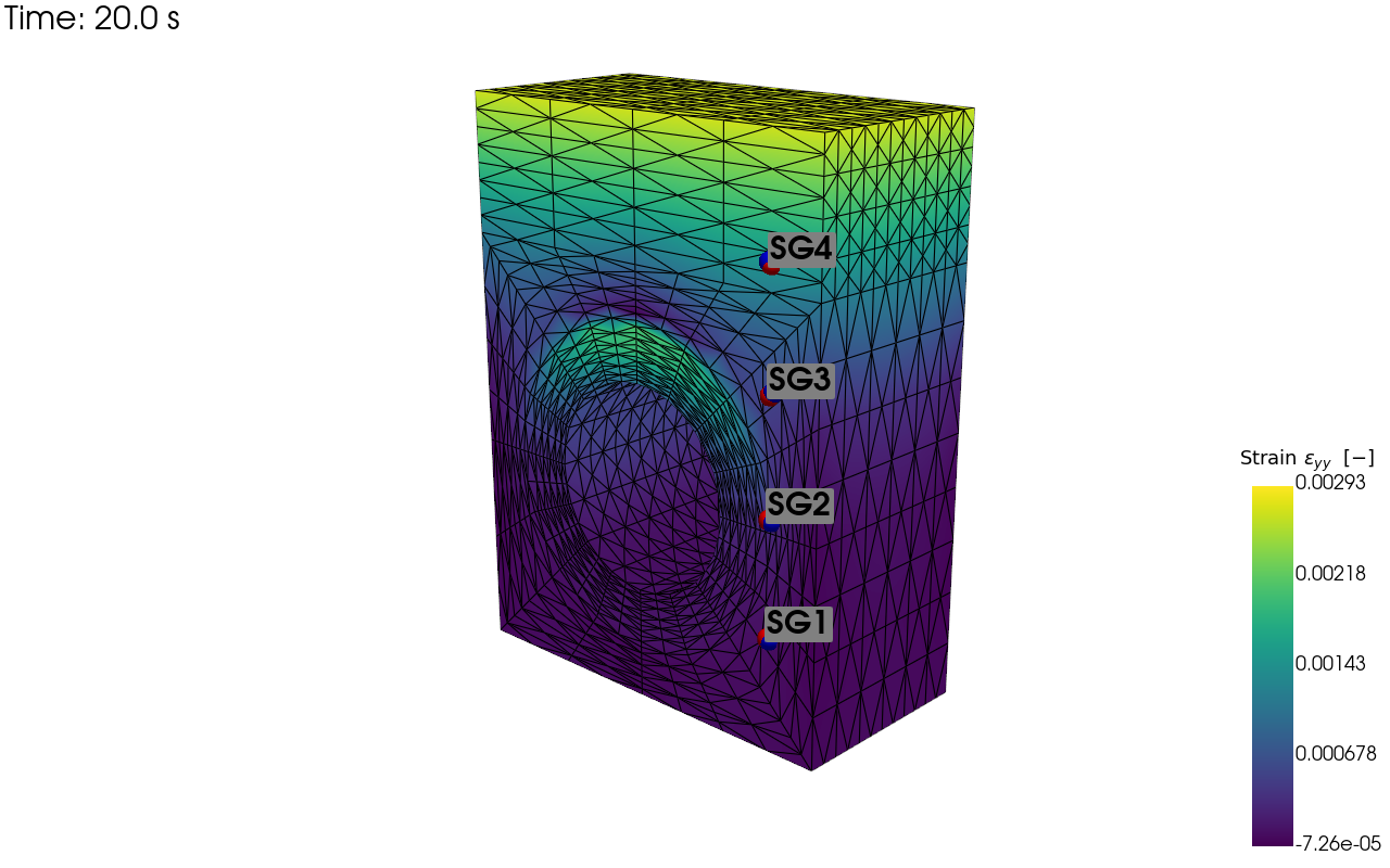
pert_sens_pos = exp_data[("sim_nominal","strain","pert_sens_pos")][-1,:,:]
pv_plot = sens.plot_point_sensors_on_sim(sensor_array=strain_sens,
                                         comp_key="strain_yy",
                                         time_step=-1,
                                         perturbed_sens_pos=pert_sens_pos)
pv_plot.camera_position = cam_pos

# Set to False to show an interactive plot instead of saving the figure
pv_plot.off_screen = True
if pv_plot.off_screen:
    pv_plot.screenshot(output_path/"ext_ex5b_strain_locs.png")
else:
    pv_plot.show()

# Uncomment to show interactive figure and set off_screen = False above
# pv_plot.show()

Visualisation of the virtual strain sensor locations:

for kk in sim_data_dict:
    (fig,ax) = sens.plot_exp_traces(
        exp_data,
        comp_ind=0,
        sens_key="temp",
        sim_key=kk,
        descriptor=sens.DescriptorFactory.temperature(),
    )

    save_fig: Path = output_path/f"ext_ex5b_traces_{kk}_temp.png"
    fig.savefig(save_fig,dpi=300,bbox_inches="tight")

Simulated temperatures traces for input physics simulation 0:

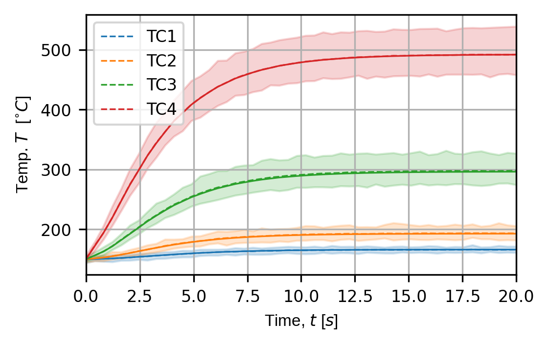
Simulated temperature traces for input physics simulation 1:

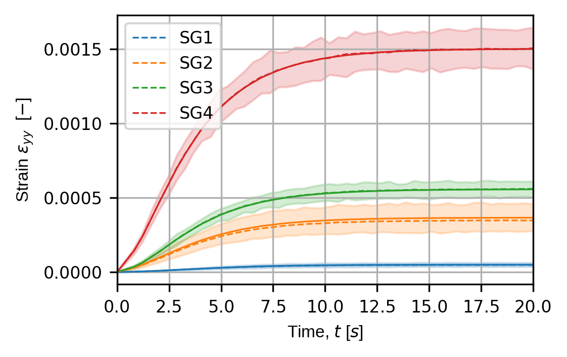
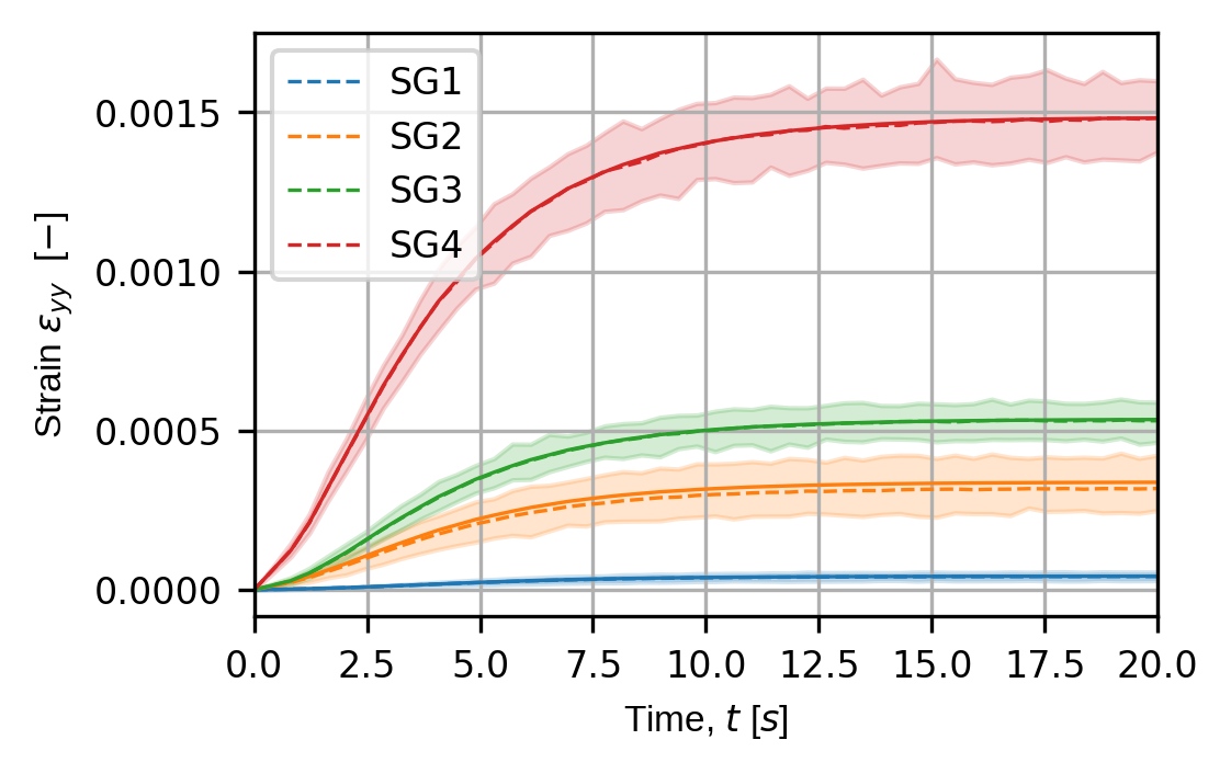
for key_sim in sim_data_dict:
    for ii,key_strain in enumerate((strain_norm_keys+strain_dev_keys)):
        (fig,ax) = sens.plot_exp_traces(
            exp_data,
            comp_ind=ii,
            sens_key="strain",
            sim_key=key_sim,
            descriptor=sens.DescriptorFactory.strain(sens.EDim.THREED)
        )

        save_fig: Path = (output_path
            /f"ext_ex5b_traces_{key_sim}_{key_strain}.png")
        fig.savefig(save_fig,dpi=300,bbox_inches="tight")

Simulated strain traces for input physics simulation 0:

Simulated strain traces for input physics simulation 1:

# Uncomment this to display the sensor trace plot
# plt.show()