HRDIC

This example walks through how a user might setup a DIC calculation for large displacment images, which are often found in micromechanics. The images used in this example are 10000x10000 pixels so you’ll need to download them from a seperate location. This example assumes the files are in the same directory/folder as the code.

Images can be downloaded here.

# pyvale modules
import pyvale.dic as dic
import matplotlib.pyplot as plt
import numpy as np

Because of the size of the images, we’ll avoid using the interactive GUI for this example. We’ll create an ROI mask that is the same size as the images using the roi.rect_boundary command. If you know that pixels along a certain edge will go outside the image bounds post deformation, then excluding them from the ROI will prevent the DIC engine from trying to correlate subsets in the reference image are not present in the deformed image.

roi = dic.RegionOfInterest(ref_image="ref.tiff")
roi.rect_boundary(left=0,right=0,top=0,bottom=0)

We’ll also chose a seed location. We’ve picked this at the centre of the image because this approximate area will be displaced the least.

roi.seed = [5000,5000]

We can then run the DIC engine using our ROI mask and seed location.

dic.calculate_2d(reference="ref.tiff",
                 deformed="def.tiff",
                 roi_mask=roi.mask,
                 seed=roi.seed,
                 subset_size=31,
                 subset_step=15,
                 max_displacement=1000,
                 fft_mad=True,
                 fft_mad_scale=3.0,
                 correlation_criteria="ZNSSD",
                 shape_function="AFFINE",
                 threshold=0.8,
                 output_basepath="./")

There’s a couple of things to pay attention to here:

• max_displacement: Sets the assumed maximum displacment. It is better to overestimate rather than underestimate this value

• fft_mad and fft_mad_scale: These remove outliers by calculating a Mean Absolute Deviation (MAD) at each stage of the FFT windowing and prevent the propagation of incorrect rigid body estimates down through the window sizes. The mad scale value determines how strict the outlier removal is - larger values of make the criterion more permissive, whereas smaller values more aggressively suppress deviations.

• threshold: Sets the minimum correlation coefficient value for a subset to be considered a good match. Any correlation coefficients less than this value will not be present in the results. If you want to have all values present in the output, you can set output_below_threshold=True.

This might take some time to run depending on the amount of available threads! You can manually set this with the num_threads argument.

The results can be imported in a standard way:

dic_files = "dic_results_*.csv"
dicdata = dic.import_2d(data=dic_files)

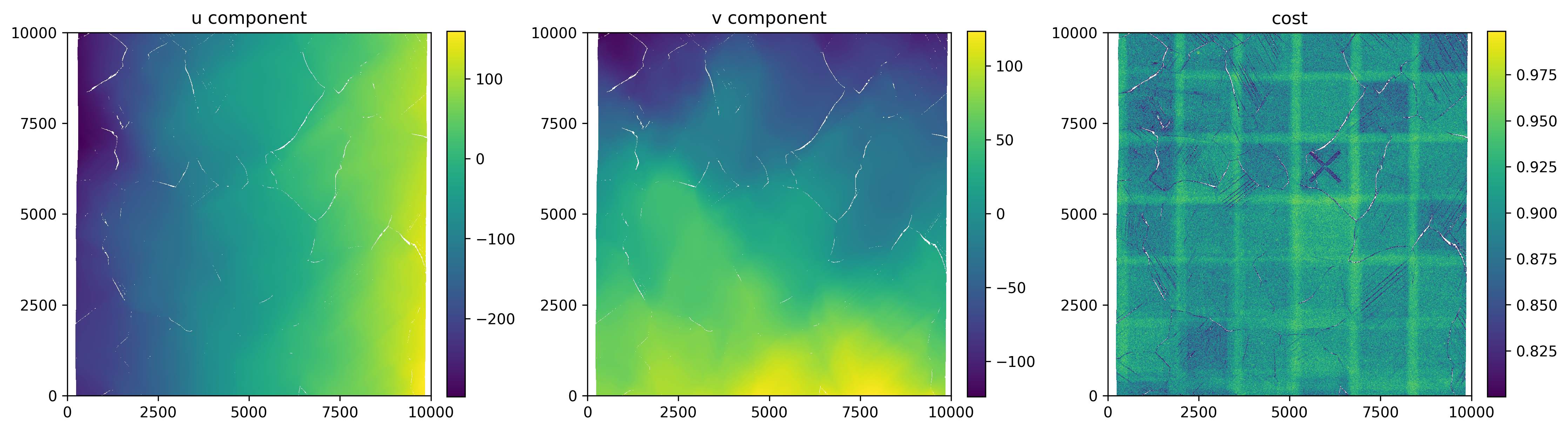
And finally a simple plot of the displacements and correlation coefficient.

fig, axes = plt.subplots(1, 3, figsize=(15, 10))
axes = axes.flatten()

# First deformation image
im1 = axes[0].pcolor(dicdata.ss_x, dicdata.ss_y, dicdata.u[0])
im2 = axes[1].pcolor(dicdata.ss_x, dicdata.ss_y, dicdata.v[0])
im3 = axes[2].pcolor(dicdata.ss_x, dicdata.ss_y, dicdata.cost[0])

# Titles
axes[0].set_title('u component')
axes[1].set_title('v component')
axes[2].set_title('cost')

# Axis ticks
ticks = np.arange(0, 10001, 2500)
for ax in axes:
    ax.set_aspect('equal')
    ax.set_xlim(0, 10000)
    ax.set_ylim(0, 10000)
    ax.set_xticks(ticks)
    ax.set_yticks(ticks)


# Colorbars
fig.colorbar(im1, ax=axes[0], fraction=0.046, pad=0.04)
fig.colorbar(im2, ax=axes[1], fraction=0.046, pad=0.04)
fig.colorbar(im3, ax=axes[2], fraction=0.046, pad=0.04)

plt.tight_layout()
plt.show()