DIC User Guide¶

This page should be conisered a guide to the core DIC user interactions and useful tips and tricks for getting good results in a reasonable amount of time. Specific examples can be found in the Examples section. If you are after a runthrough of the mathematics of the DIC engine, you can find that in the DIC Theory Overview.

Importing the DIC modules¶

After installing Pyvale, you’ll need to importing the relevent modules before going any further. We like to import the modules in the following way:

import pyvale.dic as dic
import pyvale.strain as strain

The Pyvale DIC workflow¶

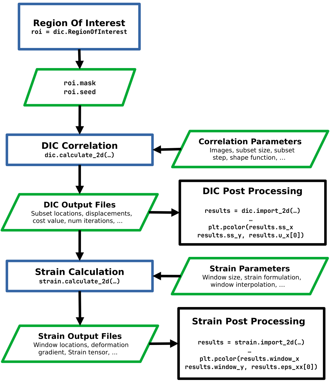
Region Of interest (ROI) Selection¶

Basic Selection¶

For any DIC calculation the user must first specify the region of interest (ROI) for their calculation. You can either use Pyvale (see the first DIC example for a detailed walkthrough), or, you can create it using Numpy. Basic approaches are summarized below:

Interactive ROI Pyvale

roi = dic.RegionOfInterest(ref_image="./ref_img.tiff") # initialization
roi.interactive_selection(subset_size=31)  # ROI GUI will launch

dic.calculate_2d(
    ...,
    roi=roi.mask,
    seed=roi.seed,
    ...,
)

Programmatic ROI Pyvale

roi = dic.RegionOfInterest(ref_image="./ref_img.tiff") # initialization
roi.rect_boundary(left=100,right=100,bottom=100,top=100) # exclude a 100 pixel boundary

dic.calculate_2d(
    ...,
    roi=roi.mask,
    seed=[500, 500],  # seed at centre of image
    ...,
)

Programmatic ROI Numpy

arr = np.zeros((1000, 1000), dtype=bool)  # image is 1000x1000
arr[100:900, 100:900] = True  # Exclude a 100 pixel boundary

dic.calculate_2d(
    ...,
    roi=arr,
    seed=[500, 500],  # seed at centre of image
    ...,
)

Behind the scenes dic.RegionOfInterest initializes roi.mask as a np.ndarray with the same dimensions as the reference image. You can then manipulate it as you would with any 2D Numpy array before passing to the DIC engine.

Defining a ROI with a YAML file¶

Another option is to use a YAML file for the ROI. When using roi.interactive_selection you can save and open ROI configurations easily within the GUI. In most cases, it will be easier to create and save the ROI YAML using the GUI and use that for all future calculations. It will also give you a sense of how the YAML is structured.

Each entry in the YAML file describes a specific ROI object with a specific type. The ROI shape can be specified with:

RectROI
CircleROI
PolyLineROI

For each ROI shape, you must also specify the Boolean flag add which indicates whether the ROI shape is being added (true) or subtracted (false) from the mask.

There are shape specific fields:

pos: For rectangular, circular, and seed ROIs: the top-left or center position as [x, y].
size: For RectROI and SeedROI: [width, height]. For CircleROI: diameter values (same number repeated).
points: For PolyLineROI an ordered list of [x, y] vertices defining the polyline.

The order in which they are defined in the YAML file determines the layering. The ROI object at the top of the file will be the bottom most layer. Any later additions or subtractions will be applied to previously defined ROI objects.

You can also specify the seed location using SeedROI. This requires the same arguments as RectRoi. Ensure that this has been configured with add: true and the width and height fields for size are identical.

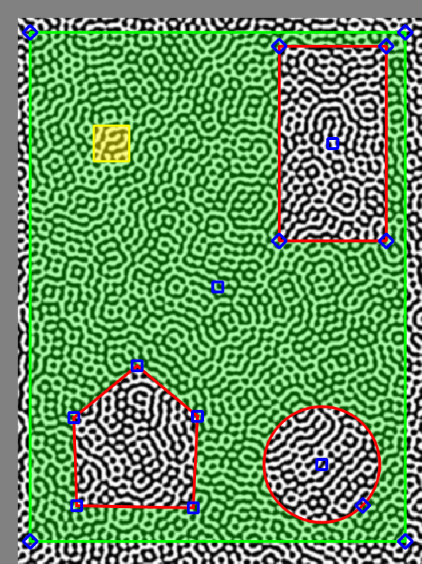
An example of an ROI configured in YAML side-by-side with it loaded into the ROI GUI can be found below:

- type: RectROI
  pos:
  - 34
  - 37
  size:
  - 433
  - 588
  add: true
  - type: RectROI
  pos:
  - 322
  - 53
  size:
  - 123
  - 225
  add: false
  - type: CircleROI
  pos:
  - 371
  - 536
  size:
  - 133
  - 133
  add: false
  - type: PolyLineROI
  points:
  - - 158
    - 422
  - - 85
    - 482
  - - 88
    - 584
  - - 222
    - 586
  - - 227
    - 480
  add: false
  - type: SeedROI
  pos:
  - 108
  - 145
  size:
  - 41
  - 41
  add: true

Performing a correlation¶

The next step is to perform a correlation with the dic.calculate_2d function. There are a few arguments that must be passed. These are the rference and deformed images, the roi mask and seed, as well as the subset size and subset step:

dic.calculate_2d(
     reference=ref_image, # Can be str | pathlib.Path | np.ndarray
     deformed=def_image,  # Can be str | pathlib.Path | np.ndarray
     roi_mask=roi.mask,   # np.ndarray
     seed=roi.seed,       # pair of intergers. Allowed as list[int] | list[np.int32] | np.ndarray
     subset_size=31,      # must be an odd number
     subset_step=15
)

All other possible arguments will have default values. See the API documentation for this function for more details.

Understanding Output files¶

The next step is to understand the output. By default the results will be saved in the users current working directory in human readable .CSV format with a filename prefix of dic_results_ followed by the name of the deformed image.

The output will have the following columns:

subset_x: X-coordinate of the center of the subset (or window) used in displacement tracking or correlation analysis.
subset_y: Y-coordinate of the center of the subset used in displacement tracking or correlation analysis.
displacement_u: Displacement in the X-direction (horizontal) calculated for the subset.
displacement_v: Displacement in the Y-direction (vertical) calculated for the subset.
displacement_mag: Magnitude of the displacement vector.
converged: Boolean flag indicating whether the displacement calculation algorithm converged for this subset.
cost: The final value of the cost function used during the displacement calculation. The reported value is always given as the ZNCC value no matter if the SSD, NSSD or ZNSSD has been chosen as the correlation function. The ZNCC is calculated with the final parameter values from the last optimizer iteration.
ftol: The final value of the function tolerance, a measure of how much the cost function changed between iterations at convergence.
xtol: The final value of the solution tolerance, a measure of how much the solution (displacement) changed between iterations at convergence.
num_iterations: The number of iterations the algorithm took to converge for this subset.

You can alter the path, delimiter and filename prefix of the output file using the arguments output_basepath, output_delimiter and output_prefix. You can also opt to save results in binary format. This can be done by setting output_binary=True.

Importing DIC Results¶

Once you have finished your correlation, you can proceed with any visualization and post-processing tools/software. Pyvale does provide the capability to read the DIC data using a single command into a dataclass that can be utilized for simple plotting. Importing data is done with the dic.import_2d command. The below highlights how to import data and create a simple plot of the displacement:

import matplotlib.pyplot as plt

dic_data = dic.import_2d(data="./dic_results_*")

# plot of vertical displacement for first deformation image.
plt.pcolor(dic_data.ss_x,
        dic_data.ss_y,
        dic_data.u_y[0]) # [image, y, x]

The import will find all files in the current working directory with that filname prefix. If you have changed output_delimiter prior to the correlation you will also need to specify the delimiter when importing the data.

Strain Calculation¶

The previous step is optional if you are wanting to perform a strain calculation. If you don’t need to do any kind of visualization or analysis, you can import DIC data and calculate strains using

Embedded DIC data Import

strain.calculate_2d(data="./dic_results_*",
   input_delimiter=",",
   window_size=5,
   window_element=9
)

Prior DIC data Import

dic_data = dic.import_2d(data="./dic_results_*", delimiter=",")

strain.calculate_2d(
   data=dic_data,
   window_size=5,
   window_element=9
)

Understanding Strain Output Files¶

Just like the DIC output, the strain output files are saved in the users current working directory in human readable .CSV format with a filename prefix of strain_ followed by the name of the deformed image.

The output will have the following columns:

window_x: X-coordinate of the strain window center.
window_y: Y-coordinate of the strain window center.
def_grad_00: Deformation gradient component, $F_{00}$.
def_grad_01: Deformation gradient component, $F_{01}$.
def_grad_10: Deformation gradient component, $F_{10}$.
def_grad_11: Deformation gradient component, $F_{11}$.
eps_00: Strain tensor component :math:`eps_{00} (normal strain in x-direction).
eps_01: Strain tensor component :math:`eps_{01} (shear strain xy).
eps_10: Strain tensor component :math:`eps_{10} (shear strain yx).
eps_11: Strain tensor component :math:`eps_{11} (normal strain in y-direction).

Importing Strain Data¶

Importing Strain data is done with the strain.import_2d command. The below highlights how to import data and create a simple plot of the normal strain in the x-direction:

import matplotlib.pyplot as plt

strain_data = strain.import_2d(data="./dic_results_*")

# plot of vertical displacement for first deformation image.
plt.pcolor(strain_data.window_x,
           strain_data.window_y,
           strain_data.eps_xx[0]) # [image, y, x]

DIC with Large Images/Displacements¶

Setting a Maximum Displacement¶

Typically if you are performing DIC with large displacements that will exceed well above 100 pixels, then there will be a few arguments that you will want to consider tweaking that might help to improve your results.

Firstly, it’s important to chose a max displacement value that is comfortably larger than your estimate for the final maximum displacement. For example, if you think your max displacement is roughly 300 pixels, then trying a value of 512 (powers of two help with FFT efficiency) would be a sensible option. This can be done with:

dic.calculate_2d(
     ...,
     max_displacement=512,
     ...,
)

Pyvale will always round the max_displacement value up to the next greatest power of 2. So if you select 400, it would still round to 512. Again, this is to benefit from the efficiencies of FFTs.

Enabling Outlier Removal in Multiwindow FFTCC Initialization¶

The FFTCC multiwindowing approach involves seeding smaller windows with the rigid estimates from neighbouring points in the previous larger window. This can sometimes be problematic when multiple windows are involved as incorrect estimates can be propogated through the smaller windows, leading to a wildly incorrect initial rigid estimate for the displacements.

Pyvale has a Median Absolute Deviation (MAD) outlier removal flag that, when enabled, will kill likely incorrect spikes in the rigid estimates or each FFTCC window size. This can be enabled with the following arguments when calling the DIC engine:

dic.calculate_2d(
     ...,
     fft_mad=True,
     fft_mad_scale=3.0, # <-- Default value
     ...
)

The MAD outlier removal works in the following way:

Looks at nearby subsets in a 2D neighborhood
Computes the median of their shifts
Computes the MAD (median absolute deviation)
A value is replaced if the the condition $| x − \mathrm{median}| > \mathrm{fft\_mad\_scale} \times \mathrm{MAD}$ is met. A larger fft_mad_scale is therefore more tolerant, while a smaller value kills larger deviations.

Sequential Image Loading¶

When working with a series of large images, RAM usage starts to become an important consideration. In it’s current form, Pyvale will read all images in the workflow when it starts. This isn’t a huge problem for typical DIC workflows where images are typically 10s of MBs, but will start to cause crashes with high resolution images (100s MBs.). To get around this we’d recommend placing the DIC engine call in a loop over the images. An example of which can be found below:

ref_img = "ref_00.tiff"
def_imgs = ["def_00.tiff", "def_01.tiff", "def_02.tiff", ...]

for def_img in def_imgs:

    dic.calculate_2d(
        ...,
        reference=ref_img,
        deformed=def_img,
        ...,
     )

There are plans to change this in later pyvale versions so that images are read sequentially and thus avoiding the need for any loops. Please keep an eye on the documentation for any future changes.

Selecting a Thread Count¶

Pyvale uses OpenMP for parallel calculations. Users can select the number of threads used in the DIC calculation with the num_threads argument in dic.calculate_2d:

dic.calculate_2d(
    ...,
    num_threads=<int>,
    ...,
 )

Alternatively, those on UNIX operating systems (MacoS, Linux) can set the number of threads using the OMP_NUM_THREADS environment variable. If you are using Windowos PowerShell you can use the command $env:OMP_NUM_THREADS=. It is worth noting that Pyvale will only use this value if it has not been specified with the num_threads= function argument.